The normal curve

The normal curve is a smoothed histogram shaped like a bell: most values near the mean, fewer and fewer towards both edges, the same on each side. Two numbers fix it completely: the mean (where the middle is) and the standard deviation (how wide the bell is).

Its key property: the area under the curve between two points is the share of cases that fall there, and so the probability that one random case lands there. The whole area is 1, everyone.

Klasna's spring mock math exam had scores with mean 150 and SD 15. The area between 140 and 160 is 0.495: about half of the learners scored in that 20-point band, and a learner picked at random has a 0.495 chance of being in it.

Read the area, never the height or the width. A 20-point band at the edge, say 185 to 205, holds only about 1% of the learners, although it is just as wide.

Three areas of the normal curve are worth knowing by heart. Within 1 SD of the mean lies about 68% of the area, within 2 SD about 95%, within 3 SD about 99.7%.

For the mock exam with mean 150 and SD 15: about 68% of learners scored 135 to 165, about 95% scored 120 to 180, and 99.7% scored 105 to 195.

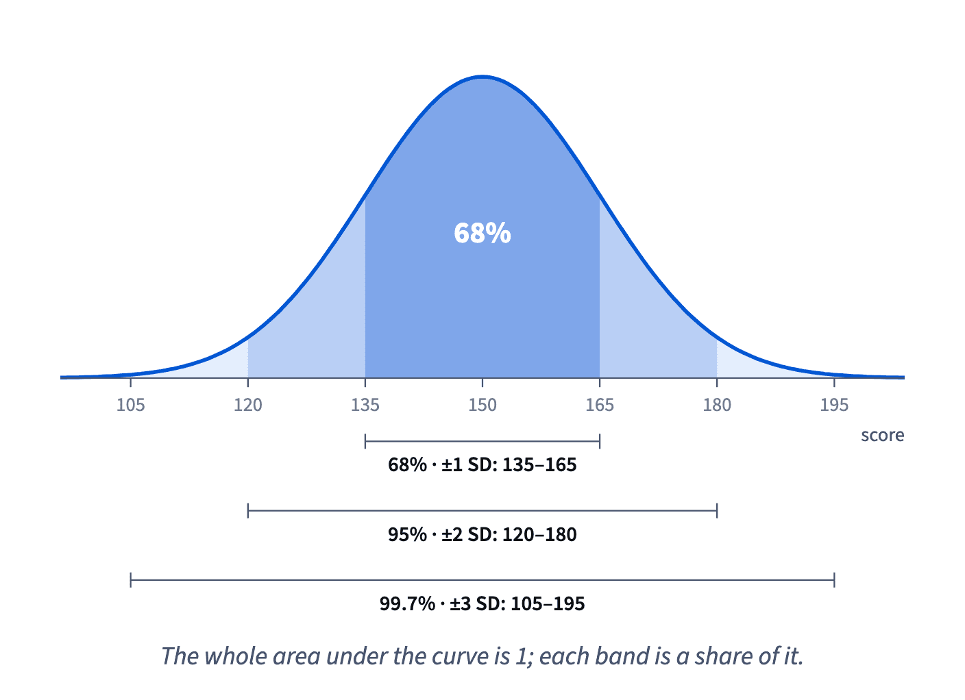
The curve is symmetric, so whatever lies outside a band splits equally between the two ends. Outside ±1 SD is 100 − 68 = 32%, so 16% scored above 165 and 16% below 135. Outside ±2 SD is 5%: 2.5% above 180 and 2.5% below 120.

That gives quick answers to "what share is above x?" whenever x sits a whole number of SDs from the mean: find the band, take what's outside it, halve it. A z-table gives the exact value, 15.9% instead of 16%, but the rule is close enough for a sanity check.

Not every metric is bell-shaped. Revenue per learner, lesson length or the number of packages bought are skewed: most values are small and a long tail stretches to one side. The 68–95–99.7 rule doesn't hold for them. A quick symptom: mean ± 2 SD reaches values that can't exist, such as a negative payment.

The curve still matters for such data, through a different door. Averages and shares measured on many people come out close to bell-shaped even when single values are skewed. The average revenue of 500 learners, or the share of 400 trial learners who buy, would form a bell if you repeated the measurement many times. That is why tests and confidence intervals can rely on the normal curve while the raw data look nothing like it.

So before using the rule, ask: is this a single value per person, or an average or share over many?

Normal curves differ only in their mean and SD, so any of them can be turned into one standard curve by measuring distance from the mean in SDs. That distance is z = (x − mean) ÷ SD, the standardizing from Standardizing: z, CV, effect size and r.

On the mock exam, a score of 180 is z = (180 − 150) ÷ 15 = 2, and a score of 171 is z = 21 ÷ 15 = 1.4. A negative z means below the mean: 135 is z = −1.

Once a value is a z, one table of areas works for every normal curve, whatever the units: exam points, minutes or a conversion rate. The 68–95–99.7 rule is that table at z = 1, 2 and 3. A test statistic in an A/B test is also a z: the measured difference divided by its standard error, so the same table turns it into a p-value.

"95% within 2 SD" is a rounded rule. The exact z that leaves 95% of the area in the middle, and so 2.5% in each tail, is 1.96. That is the number behind every 95% interval and every two-tailed test at the 5% level.

Other levels have their own cut-offs, found the same way. For 90% in the middle, 5% per tail, it is 1.645; for 99%, 0.5% per tail, it is 2.576. The rule is always: split what's left outside between the two tails, then find the z that leaves that much beyond it.

The most common slip is to put the whole 5% in each tail. That describes a 90% band, not a 95% one. Another is to think 1.96 is just a friendlier 2: it is the more precise value, and 2 is the rounding.

A confidence interval puts the 1.96 to work. An average or share measured on many people is roughly normal around the true value, with the standard error from Square roots and √n as its SD. So the measured value ± 1.96 standard errors covers the true value in 95% of such measurements.

Klasna's trial lessons: 30% bought, SE ≈ 2.3 pp. 1.96 × 2.3 = 4.5, so the interval is 30% ± 4.5, from 25.5% to 34.5%. A survey where 42% of parents want weekend lessons, with SE = 3 pp: 1.96 × 3 = 5.88, so 36.1% to 47.9%.

Three habits help. Multiply first, then add and subtract. Keep the units straight: an SE in percentage points goes with a share in percent. And report both ends, not only the centre: "42%, between 36% and 48%" says how much the survey can be trusted.

A p-value is an area too: the share of the curve at least as far out as the observed z, if there were no real effect. The question decides which tails count.

Klasna's new lesson reminder gave z = 1.87, and the area beyond 1.87 on one side is 0.031. The usual question, "is attendance different, better or worse?", counts extreme results on both sides: two-tailed p = 0.031 + 0.031 = 0.062, above 0.05. Only "is it better?" counts one tail: p = 0.031. For z = −2.10 with 0.018 per tail, the two-tailed p is 0.036; the sign doesn't matter, because the curve is symmetric.

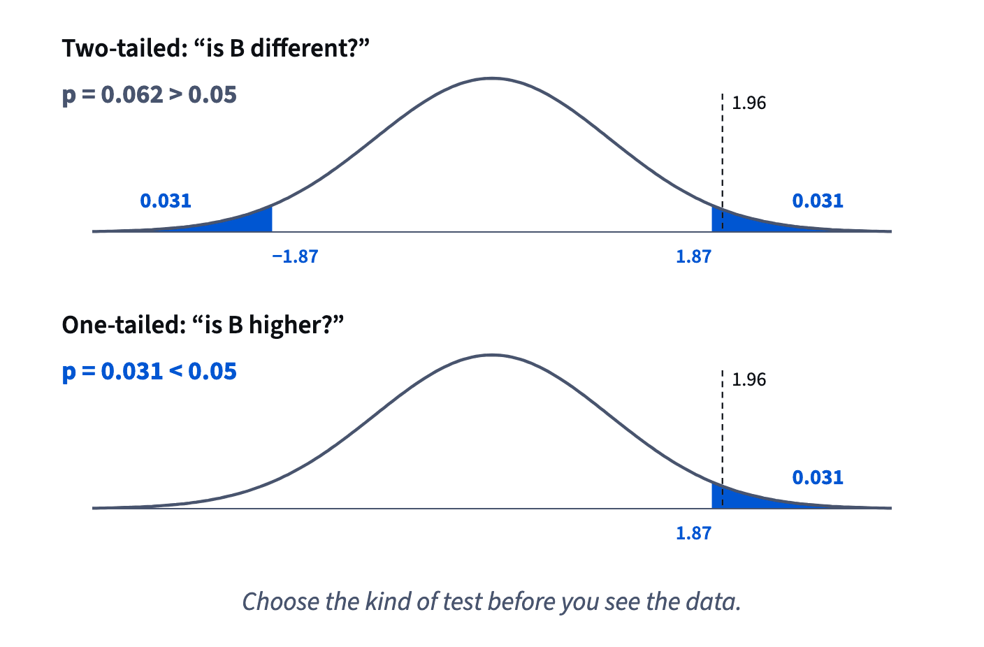
A one-tailed test is fair only if it was chosen before seeing the data and a drop would truly change nothing. Picking it afterwards, because the two-tailed p missed, doubles the real false-alarm rate. Most product tests are two-tailed.

Sample-size formulas for a test contain two z-values added and squared: n ∝ (z_{α/2} + z_β)². The first, z_{α/2} = 1.96, sets the false-alarm rate of a two-tailed 5% test. The second, z_β, sets the power: the chance to detect a real effect of the planned size. For 80% power z_β = 0.84, because 80% of the curve lies below 0.84.

Together, (1.96 + 0.84)² = 2.8² = 7.84. Asking for 90% power uses z_β = 1.28: (1.96 + 1.28)² = 3.24² = 10.50, and 10.50 ÷ 7.84 ≈ 1.34. Ten more points of power cost about a third more people, everything else equal.

Because the sum is squared, small changes in either z move the sample a lot. That is why teams agree on α and power before planning a test.

How it fits together: area is probability; z puts any normal curve on one scale; 1.96 cuts 95% in the middle, giving intervals, p-values and sample sizes. The next lesson meets the t, chi-square and F curves and computes power itself.