Standardizing: z, CV, effect size and r

A z-score says how far a value sits from the mean of its group, counted in standard deviations: z = (x − μ) ÷ σ. With sample data, use x̄ and s.

• z = 0: exactly average for the group.
• z = +2: two SDs above the mean.
• z = −1: one SD below it.

The point is the common ruler. Raw numbers from different groups can't be compared: subjects rate differently, tests differ in difficulty. Dividing by each group's own SD turns every value into "how unusual is this for its own group".

Example: English tutors average 4.5 with SD 0.1, math tutors 4.6 with SD 0.25. An English tutor at 4.7 has z = (4.7 − 4.5) ÷ 0.1 = 2.0; a math tutor at 4.8 has z = (4.8 − 4.6) ÷ 0.25 = 0.8. The lower raw rating is the more outstanding one.

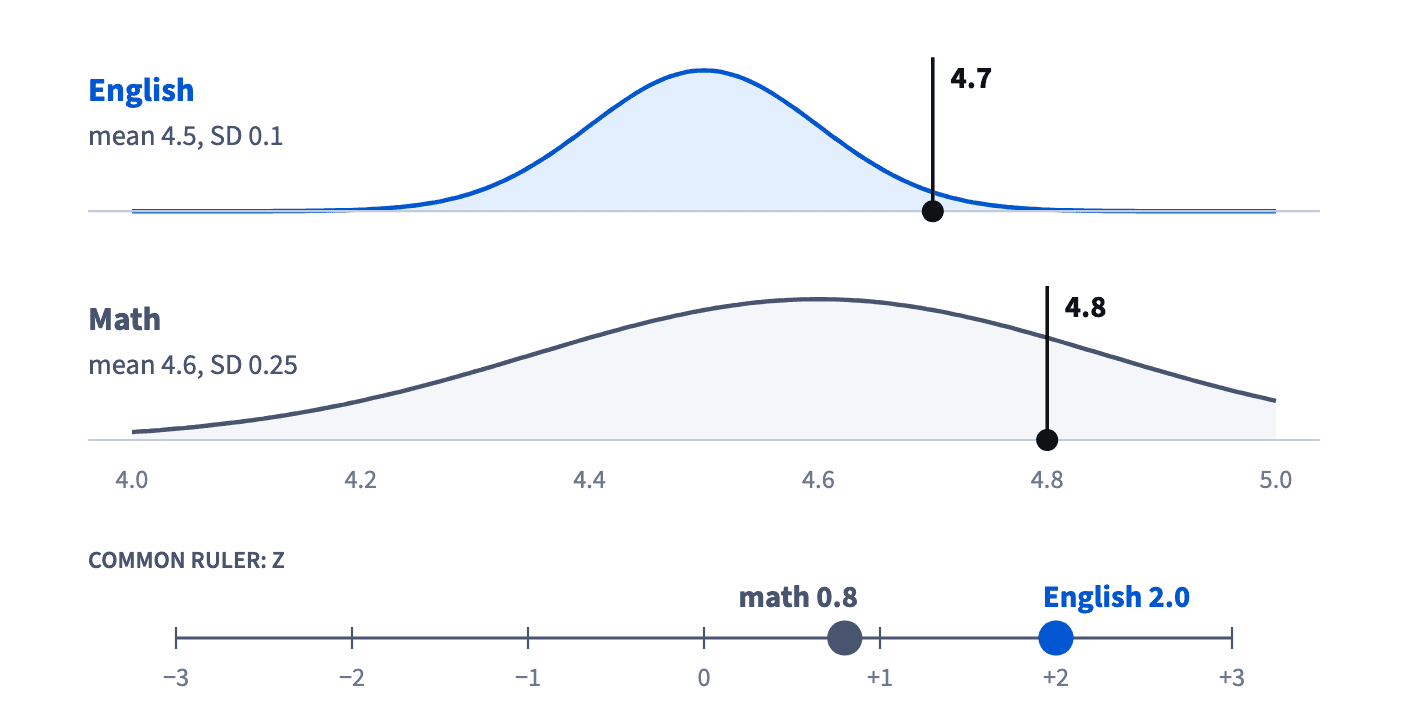
Mind the order of operations from Order of operations, ratios and multiples: subtract first, then divide. Without brackets, 4.7 − 4.5 ÷ 0.1 = −40.3, a meaningless number.

Once values are z-scores, comparisons across groups become fair, and unusual values become easy to spot.

Fair comparisons. A learner scoring 85 on a test with mean 80 and SD 10 is at z = 0.5. A learner scoring 70 on a harder test with mean 64 and SD 3 is at z = 2.0. The second did far better relative to their group, despite the lower raw score. The same logic can pick a "tutor of the term" across subjects.

Outlier checks. A common rule flags |z| ≥ 3 as suspicious: in roughly bell-shaped data, a value three or more SDs from the mean is rare. A tutor whose average rating has z = −3.2 deserves a look: a real problem or a data error.

Two cautions. z inherits whatever the mean and SD contain: one huge outlier inflates the SD and can partly hide itself. And z shows position, not certainty: z = 2 within three tutors says much less than within three hundred.

An SD of 8 lessons a week is huge for a tutor who teaches 10 lessons and small for one who teaches 100. The coefficient of variation puts spread in proportion to size: CV = s ÷ x̄, usually shown in percent.

Example: English tutors teach 40 lessons a week on average with SD 8, so CV = 8 ÷ 40 = 20%. Programming tutors teach 10 with SD 4: CV = 4 ÷ 10 = 40%. Programming has the smaller SD but is twice as unpredictable for its size.

Because the units cancel, CV compares things measured in different units: the spread of monthly spend in hryvnias against the spread of lessons or minutes.

Keep the order: SD on top, mean below. Mean ÷ SD is the upside-down version and belongs to a different idea, a signal-to-noise ratio. And read CV as "the SD is a fifth of the mean", not as a probability or a change.

CV divides by the mean, so it makes sense only when the mean is a meaningful size: for quantities that can't go below zero, such as lessons, money, minutes or users.

For numbers that can be negative, it breaks. The weekly change in bookings can be +40 one week and −35 the next; its mean may be +2 with an SD of 30. Then CV = 30 ÷ 2 = 1,500%, which says nothing about stability. If the mean drifts to −2, the CV turns negative; at a mean of exactly 0 it can't be computed at all. The trouble is the denominator, not the data.

The same caution applies to profit that can turn into a loss, to temperatures and to any score with an arbitrary zero.

What to use instead: report the SD itself in the original units ("the weekly change varies by about 30 bookings"), or compute the CV on the underlying level, bookings per week, which is always positive.

Cohen's d measures an effect against how much people differ: d = difference in means ÷ s_p, where s_p is the pooled SD of the two groups (pooled variance came up in Weighted mean and mix).

Example: a new homework format raises test scores by 6 points, and scores vary with s_p = 15. d = 6 ÷ 15 = 0.4: four tenths of an SD.

Why divide? Raw effects come in units that don't compare. +0.2 rating points and +12 minutes of practice can't be ranked as they stand; in SD units they can. That makes d useful for comparing tests and for planning them: the smaller the d you hope to detect, the bigger the test you need.

d describes size, not certainty. It doesn't grow with the sample: 100 users or 100,000 give about the same d for the same effect. And don't attach fixed labels such as "small" or "large" without context: a d of 0.1 on revenue can be worth more than 0.5 on a metric nobody acts on.

Test statistics are standardized too. t = difference ÷ its standard error: the signal measured in units of noise. You met the paired version in Square roots and √n. A t of 3 means the difference sits three SEs away from zero.

t and d divide by different things. d divides by the spread between people, s_p, which doesn't shrink with more data. t divides by the SE, s ÷ √n, which does. So t grows roughly with √n even when the effect stays the same.

With 100,000 users per group, a lift of d = 0.03 gives t ≈ 0.03 × √50,000 ≈ 6.7: almost certainly real, and also tiny. A small pilot can show the opposite: d = 0.5 with t = 1.2, a possibly large effect measured too roughly to trust.

So report both. t, or the p-value built from it, answers "is it real?"; d answers "is it big?".

Covariance tells whether two metrics move together: positive when high values of one come with high values of the other, negative when they go opposite ways. Its size, though, depends on the units: measure homework in minutes instead of hours and the covariance grows 60 times.

Dividing by both SDs removes the units: r = cov ÷ (s_x · s_y). The result, the correlation coefficient, always lies between −1 and 1.

Example: homework hours and test scores have cov = 24, s_x = 3 hours and s_y = 10 points. r = 24 ÷ (3 × 10) = 0.8, a strong positive link.

Mind the product in the denominator: multiply the two SDs first, then divide. Working left to right, 24 ÷ 3 × 10 = 80, an impossible r. If you ever get |r| > 1, something upstream is wrong.

r measures straight-line links only, and it doesn't say what causes what: more homework and higher scores may both come from more motivated learners.

The sign of r gives the direction of a link; its size without the sign, |r|, gives the strength.

• r near +1: points rise together, tightly.
• r near 0: no straight-line pattern, a shapeless cloud.
• r near −1: one falls as the other rises, tightly.

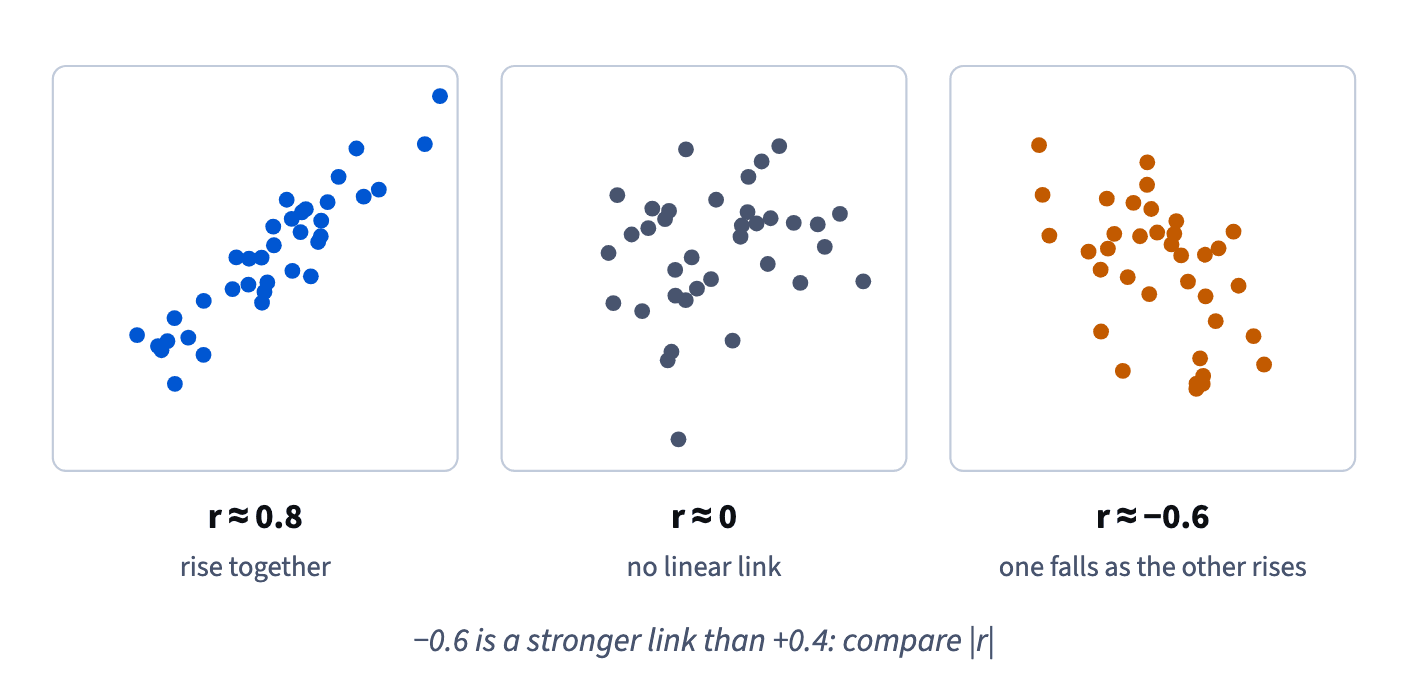
So r = −0.72 is a stronger link than r = 0.60: compare 0.72 with 0.60. The minus only says that, for example, more days since the last lesson go with a lower chance of booking again.

How it fits together: this module built spread from squares (variance), roots (SD and SE) and Pythagoras, and this lesson divides by spread to put numbers on one scale: z, CV, d, t and r. Module 5 turns to lines and models: what a slope means and how a total splits into parts.