Square roots and √n: SD and the standard error

A variance is measured in squared units: the five learners' variance of 14.5, from Why we square, is in "lessons squared", which no one can picture. The standard deviation takes the square root and brings the unit back: s = √s² = √14.5 ≈ 3.81 lessons. Think of the variance as the area of a square; the SD is its side.

Read the SD as a typical distance of a value from the mean. With a mean of 8 lessons and s ≈ 3.8, most learners are within about four lessons of 8, on either side. The population version works the same way: σ = √σ².

Two checks keep the arithmetic honest. Square your answer and you should get the variance back: 3.81 × 3.81 ≈ 14.5. And the SD can never be negative or larger than the whole range of the data.

In a spreadsheet, STDEV.S is the square root of VAR.S, and STDEV.P the square root of VAR.P.

The standard deviation and the standard error answer different questions, and mixing them up is one of the most common reporting slips.

• SD: how much individual values differ. "8 ± 3.81 lessons" is a fair description of the five learners: a typical one is about 4 lessons from the mean.
• SE: how much the mean of a sample would wobble if you drew another sample of the same size. For n > 1 it's always smaller than the SD, and it shrinks as the sample grows; the SD doesn't.

So "mean ± SD" describes how people spread, and it is not a confidence interval. Reading 8 ± 3.81 as "the true average is between 4.2 and 11.8" mixes the two: that range is where typical learners are, not where the average is. An interval for the average is built from the SE (module 7 shows how).

In a report, always say which one you show: "SD 3.8" or "SE 1.7", never a bare "± 3.8".

A sample mean is itself a random number: draw another five learners and you get a different mean. The standard error measures how much it would wobble: SE = s ÷ √n.

Why √n and not n? Random errors partly cancel: some values land above the mean, some below. The cancelling grows with the square root of the sample size, not with the size itself. For the five learners, s = 3.81 and √5 ≈ 2.24, so SE ≈ 1.70 lessons. With 20 learners and the same spread, √20 ≈ 4.47 and SE ≈ 0.85.

Notice what changes and what doesn't. More data leave the SD roughly where it was (learners don't become more alike), but the SE keeps falling.

Order of work: take √n first, then divide. Ratings with s = 15 points averaged over n = 25 give SE = 15 ÷ 5 = 3 points: single ratings vary by about 15, their average by about 3.

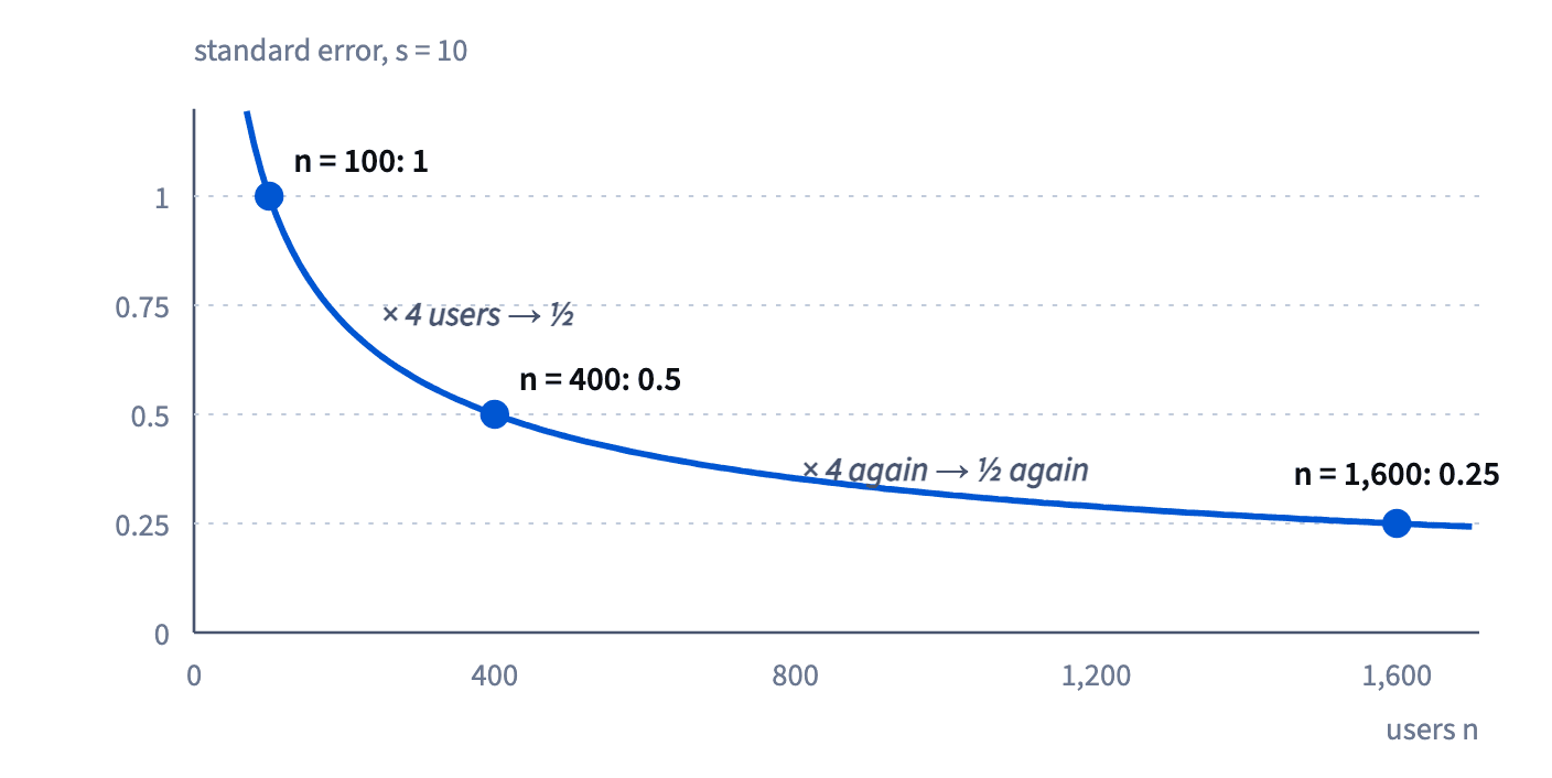
Because SE = s ÷ √n, the error falls with the square root of the sample size, so extra data get steadily less rewarding.

• 4 times the data → √4 = 2 → the error halves.
• 100 times the data → √100 = 10 → the error falls tenfold.
• 2 times the data → √2 ≈ 1.41 → the error falls by only about 29%.

With s = 10: at n = 100 the SE is 1.0, at n = 400 it's 0.5, at n = 1,600 it's 0.25. Each halving costs four times the users of the step before. The first hundred users teach you a lot; every next batch, less.

This is the arithmetic behind every "can't we just run the test a bit longer?" talk. Doubling a test's length doesn't halve its error: you'd have to make it four times as long. It also works the other way: a quarter of the data doubles the error.

For a share, such as a conversion rate, there is no separate s to plug in: the spread comes from p itself. A yes/no outcome with share p has variance p(1 − p), so

SE_p = √(p(1 − p) ÷ n).

Worked example: 5% conversion measured on n = 1,900 users. p(1 − p) = 0.05 × 0.95 = 0.0475. Divided by 1,900: 0.000025. Square root: 0.005, that is 0.5 percentage points.

Three habits keep it right:

• write p as a decimal inside the formula (0.05, not 5) and convert the result to percentage points at the end;
• divide by n before taking the root, not after;
• remember that p(1 − p) is largest at p = 0.5, so shares near 50% are the noisiest to measure (p and 1 − p in module 7 returns to this).

Read the result in percentage points: an SE of 0.005 on a 5% rate means 0.5 pp, not 0.5%.

The minimum detectable effect (MDE) is the smallest true lift a test can reliably detect. With the usual settings it is about 2.8 standard errors: MDE ≈ 2.8 × SE. Where the 2.8 comes from is a topic for module 7; here we only use it.

Because the MDE is always the same number of SEs, it inherits the √n rule. Say 1,500 users per group give an MDE of 3 pp. Then:

• 6,000 per group (4×) give 1.5 pp;
• 3,000 per group (2×) give about 3 ÷ 1.41 ≈ 2.1 pp, not 1.5 pp;
• 375 per group (¼) give 6 pp.

Halving the effect you want to see quadruples the sample. That's why "let's look for a smaller lift" is an expensive sentence. Decide first what the smallest lift worth acting on is, then size the test for it, not the other way round.

When the same people are measured twice, before and after a training or last month and this month, compare each person with themselves. Work with the differences d = after − before, and the √n rule applies to them:

• d̄: the mean difference;
• s_d: the standard deviation of the differences;
• SE = s_d ÷ √n;
• paired t = d̄ ÷ SE: how many standard errors the mean change sits from zero.

Example: 16 Klasna tutors were rated before and after a training. The mean change is d̄ = 0.3 points with s_d = 0.4. SE = 0.4 ÷ √16 = 0.1, so t = 0.3 ÷ 0.1 = 3: the change is three standard errors from zero, hard to put down to luck.

The slip to avoid is using the spread of the raw ratings instead of the spread of the differences. Pairing removes the differences between tutors, so s_d is usually much smaller, and that is the whole point of pairing.

The formula s ÷ √n assumes the population is huge next to the sample. When the sample is a big part of a small population, less is left uncertain, and the SE shrinks by the finite-population correction: √((N − n) ÷ (N − 1)).

Surveying 400 of Klasna's 1,120 learners: √(720 ÷ 1,119) = √0.643 ≈ 0.80, so the SE is 20% smaller than the plain formula says. Surveying 400 of a million, the factor is about 1 and can be ignored. A common rule of thumb: bother only when the sample is more than about 5% of the population.

How it fits together: the square root turns variance into the SD; dividing by √n turns the SD into the standard error of a mean or a share; the MDE and the paired t are built on that SE. The next lesson shows how errors and distances add up as squares.