Several variables

A model can take several inputs at once: ŷ = b₀ + b₁x₁ + b₂x₂ + … + bₖxₖ, or b₀ + Σbⱼxⱼ with the sum sign from The Σ sign: sums, limits and running totals. ŷ ("y-hat") is the model's prediction, not a measured value.

Each piece reads like the line in The linear function:

• b₀ is the start, the prediction when every x is 0;
• each bⱼ is a slope for its own input, holding the others fixed.

Klasna's marketing model for new families a month is ŷ = 40 + 0.15·spend + 25·exam, with spend in thousand UAH and exam = 1 in exam months. One more thousand of spend adds 0.15 families whatever the month; 100 thousand more add 15.

Always read a coefficient with the unit of its input. 0.15 looks tiny because the unit is a thousand hryvnias; with spend in plain hryvnias the same effect would read 0.00015. A coefficient's size says nothing about importance until you know its unit and the usual range of its input.

To get a prediction, substitute every input and add the terms. For an exam month with spend of 90 thousand UAH: ŷ = 40 + 0.15 × 90 + 25 × 1 = 40 + 13.5 + 25 = 78.5 families. In a month without exams the exam term is 0, so 53.5.

A prediction of 78.5 families is an average expectation, not a promise; real months scatter around it.

Be careful with b₀. Read literally, 40 means 40 families with no spend at all, outside exam season. But every month in Klasna's data had some spend, so zero lies outside what the model has seen. Predicting far outside the data, at a spend of 0 or of 2 million, stretches a straight line where nobody checked that it stays straight. Often b₀ only anchors the line inside the observed range.

Keep inputs in the model's units: entering spend as 90,000 instead of 90 would predict 13,565 families for an exam month.

Some inputs aren't amounts but yes/no facts: an exam month or not, a group lesson or not, a new or a returning user. A model codes them as 0/1 variables (dummy variables): 1 when the fact holds, 0 when it doesn't.

The coefficient then reads as a shift. In ŷ = 40 + 0.15·spend + 25·exam, switching exam from 0 to 1 adds 25 families at the same spend; when exam = 0, the term 25·0 vanishes. So the model draws two parallel lines, the exam line 25 families above the other.

Three readings to avoid:

• 25 is not a percent: it's in the units of ŷ, families;
• it is not a slope: it doesn't grow with spend;
• it is a comparison with the category coded 0, the baseline, here months without exams.

A fact with more than two values, such as four seasons, needs one 0/1 variable per category except the baseline: three for four seasons.

Sometimes two inputs work together. In exam season parents may react to ads more strongly, so the same thousand brings more families. A model captures that with an interaction term, a product of two inputs: ŷ = 40 + 0.15·spend + 25·exam + 0.10·spend·exam.

In other months exam = 0 and the interaction vanishes: each thousand brings 0.15 families. In exam months the slope of spend becomes 0.15 + 0.10 = 0.25.

Without the interaction, exam months were a parallel line 25 higher. With it, the exam line is also steeper, and the gap grows with spend: 25 at zero spend, 25 + 0.10 × 100 = 35 at 100 thousand.

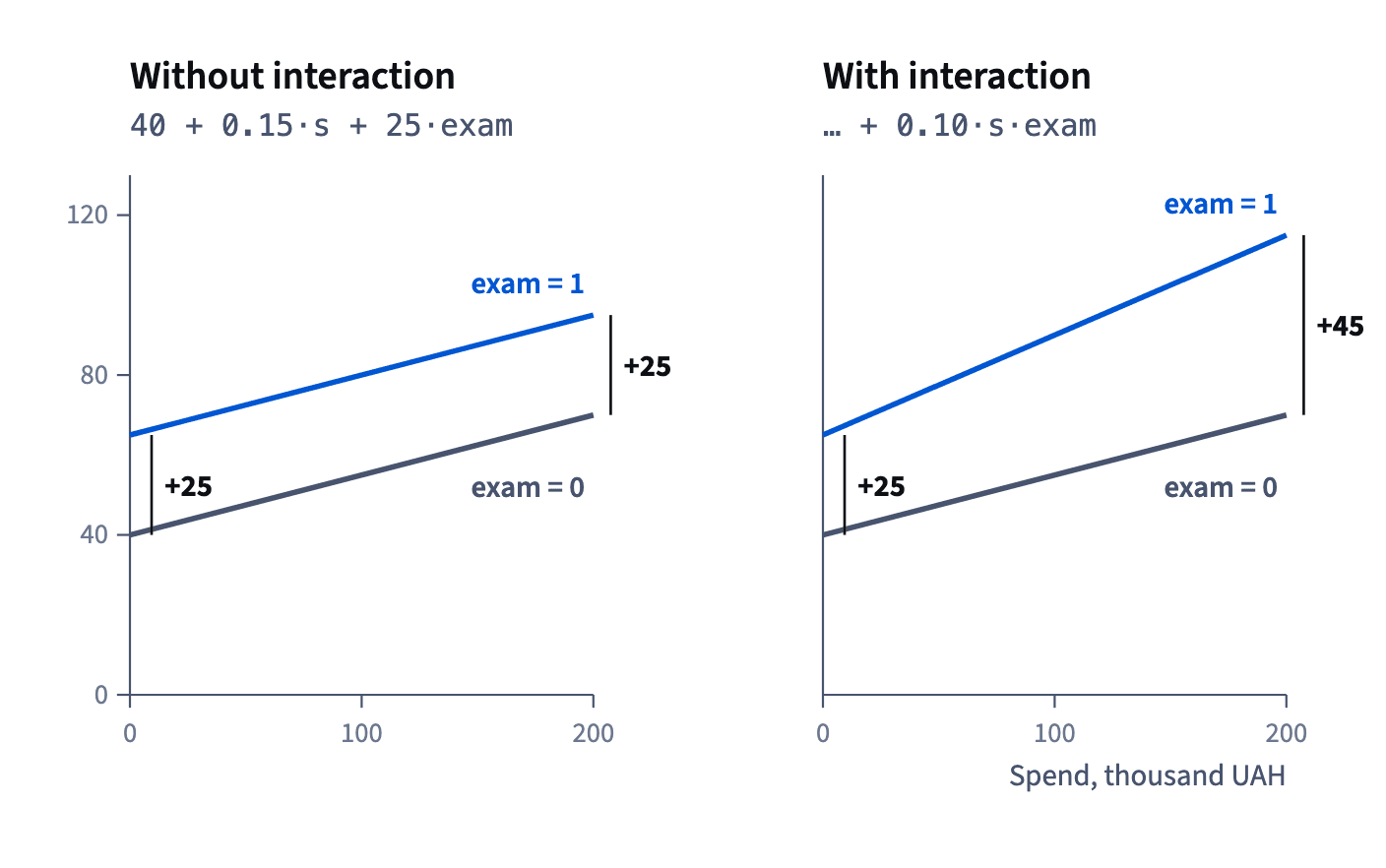
So in a model with interactions "the effect of spend" has no single answer. Report it case by case ("0.15 families per thousand outside exams, 0.25 in exam months") instead of quoting one coefficient as if it held everywhere.

Finance builds forecasts from the things that cause the result, called drivers. Klasna's monthly operating profit is

OP = L · (0.975·P − T − V·FX) − F,

with L the lessons, P the price, 0.975 what remains after the 2.5% payment fee, T the tutor payout, V video and AI per lesson in USD, FX the dollar rate and F the fixed costs.

Read it from the inside out, as the order of operations in Order of operations, ratios and multiples says. The bracket is the contribution per lesson. With P = 650, T = 415, V = 0.75 and FX = 42: 0.975 × 650 − 415 − 0.75 × 42 = 633.75 − 415 − 31.50 = 187.25 UAH. Then multiply by lessons and subtract fixed costs.

The point of this shape is that each driver has an owner and a way to check it: pricing owns P, the tutor team owns T, finance watches FX. A forecast written as one number gives nothing to argue with; a driver forecast shows which assumption moved.

A driver forecast is a chain of products, so build it one link at a time. Lessons themselves come from two drivers: L = learners × lessons per learner. October: 1,010 × 6.5 = 6,565 lessons.

Then contribution = L × contribution per lesson = 6,565 × 187.25 = 1,229,296.25 UAH, and OP = 1,229,296.25 − 1,062,000 = 167,296.25 UAH.

Two habits keep it right. Compute the per-lesson bracket once and reuse it, instead of multiplying each driver by L separately and losing a term on the way. And keep the units in view: learners × lessons per learner = lessons; lessons × UAH per lesson = UAH. If the units don't end in UAH, a link is missing.

Notice how small the result is next to its parts: 167 thousand of profit out of 1.23 million of contribution. That thin leftover is why a small change in a big driver moves profit so much, which a sensitivity test measures.

To find which driver matters, run a sensitivity test: move one driver by the same step, say 10%, keep all the others, and record how far the result moves. Then sort by size.

For October, with a profit of 167,296 UAH:

• price +10%: 0.975 × 65 × 6,565 ≈ +416,057;
• tutor payout +10%: 41.5 × 6,565 ≈ −272,448;
• lessons +10%: 656.5 × 187.25 ≈ +122,930;
• fixed costs +10%: −106,200;
• dollar rate +10%: 0.75 × 4.2 × 6,565 ≈ −20,680.

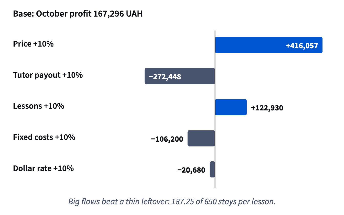
Sorted, the bars form a "tornado" chart. Big flows such as price and payout beat the small leftover, even though the leftover is what you care about: a 10% price error is worth more than twice the month's whole profit.

Two pitfalls: ranking drivers by their own size instead of their effect on the result, and moving them by different steps (10% for one, 50 UAH for another), which makes the bars incomparable.

A sensitivity test moves one driver at a time to show where to look. A scenario moves several drivers together into one consistent story, to show what could happen.

A weak-year scenario for Klasna might combine fewer learners, a price cut to keep them and a pricier dollar, because such things tend to arrive together. A strong year: more learners, a steady price, more lessons each. Every scenario is computed with the same driver formula, just with all its assumptions changed at once.

The two answer different questions, so use both. Sensitivity says which assumptions deserve a week of checking; scenarios give the plan a range and a story to act on. Don't add up sensitivity bars to get a scenario: drivers multiply each other, so a combined move isn't the sum of single moves.

How it fits together: a model with several inputs is a slope per input, read with the others fixed; 0/1 variables shift it, interactions tilt it, drivers chain it, and sensitivity and scenarios show what matters. The next lesson splits a total into parts: sums of squares, R² and plan versus actual.