Pythagoras in statistics: distances and errors in quadrature

In a right triangle, c² = a² + b²: legs of 3 and 4 give a diagonal of √(9 + 16) = 5. Statistics uses this school rule far more often than it admits, and the first place is distance.

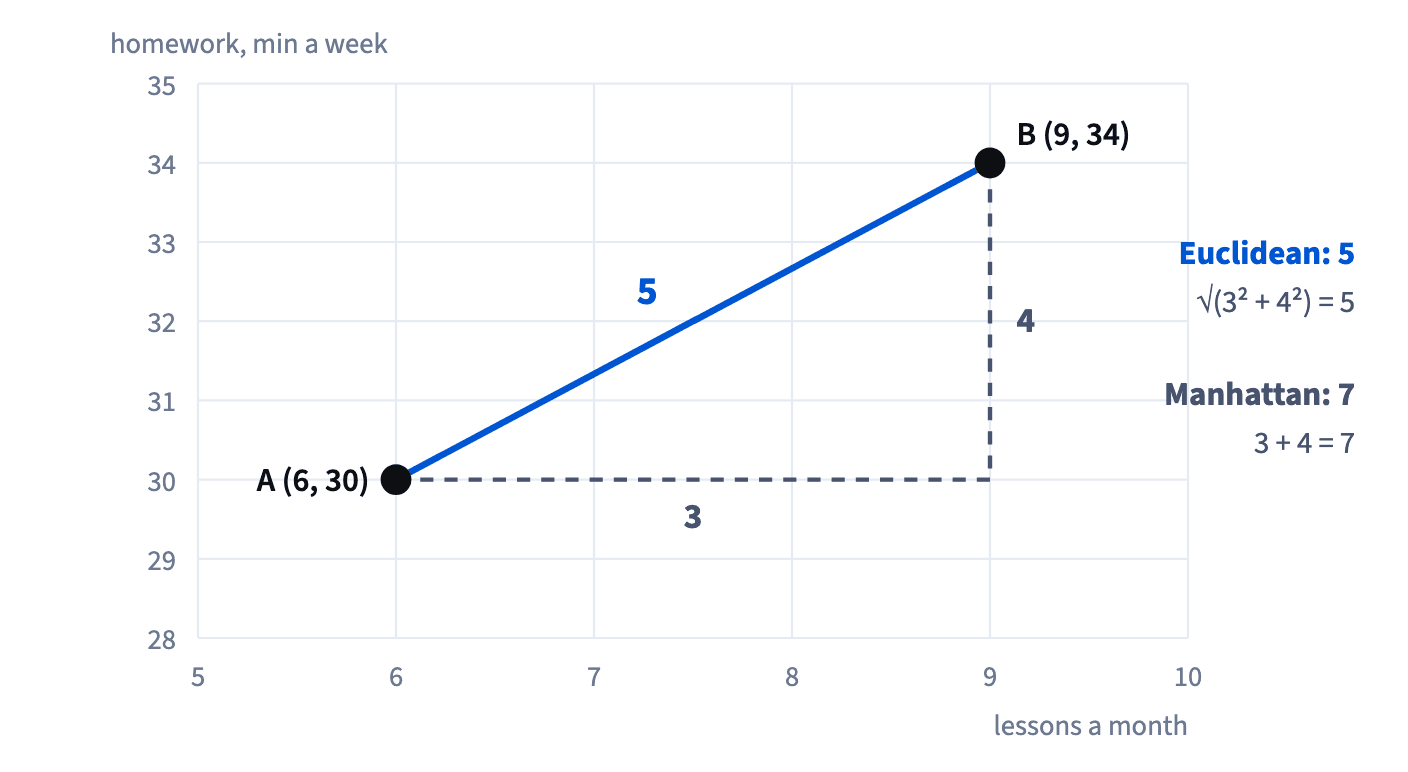
Describe each learner by numbers, for example lessons a month and homework minutes a week. A is (6, 30), B is (9, 34). The differences, 3 and 4, are the legs, and the straight-line Euclidean distance is the diagonal: √(3² + 4²) = 5.

With more features only the number of squares grows: d = √Σ(xᵢ − yᵢ)². Subtract feature by feature, square, add, and take one root at the end.

Two cautions. The root comes last: rooting each square and adding gives 3 + 4 = 7, a different measure. And the features need comparable scales: if one is in minutes and the other in lessons, the minutes dominate the sum. That's why clustering usually standardizes features first, which Standardizing in this module explains.

The Manhattan distance measures along the grid instead of across it, like walking city blocks: add up the size of each difference and ignore its sign. d = Σ|xᵢ − yᵢ|.

The bars |x| mean the absolute value: the number without its sign. |−4| = 4 and |4| = 4. Without the bars, differences in opposite directions would cancel, just as deviations from a mean do.

For learners A (6, 30) and B (9, 34): |9 − 6| + |34 − 30| = 3 + 4 = 7, against 5 along the straight line. The Manhattan distance is never shorter than the Euclidean one; the two are equal only when the points differ in a single feature.

Which one to use is a modelling choice. The Euclidean distance, through its squares, punishes one big difference more. The Manhattan distance treats every unit of difference alike, so one odd feature sways it less. Both need features on comparable scales.

The SE of a difference between two independent groups is not the sum of their SEs. Say variant A converts at 8% with SE 0.5 pp and B at 10.6% with SE 1.2 pp. The SE of B − A is

√(0.5² + 1.2²) = √(0.25 + 1.44) = √1.69 = 1.3 pp, not 1.7.

Why? The two errors are random and independent. When A happens to be measured too high, B is as likely to be too low as too high, so the errors partly cancel. What adds up exactly is the variance: 0.25 + 1.44 = 1.69. The SE, its square root, adds like the sides of a right triangle. This is called adding in quadrature.

It changes decisions. With the plain sum, the 2.6 pp gap is 2.6 ÷ 1.7 ≈ 1.5 SEs and gets waved off as noise; with the right SE it is 2.6 ÷ 1.3 = 2 SEs.

The same Pythagoras works for any sum of independent uncertain pieces, not only for test groups. If tasks run one after another and each has its own independent uncertainty σ, the uncertainty of the total is

σ_total = √(σ₁² + σ₂² + …).

Two tasks with σ = 3 and 4 days: √(9 + 16) = 5 days, not 7. Square each, add, and take one root at the end.

The total always lands above the largest piece and below the plain sum. Notice how one big piece dominates: with σ = 1, 1 and 5 days, √(1 + 1 + 25) ≈ 5.2, barely more than the biggest piece alone. To shrink a combined uncertainty, work on the largest source first; trimming the small ones hardly moves it.

Project plans, budgets built from several estimates and measurements with several error sources all combine this way, as long as the pieces are independent.

Adding in quadrature rests on one assumption: the pieces are independent, so their errors partly cancel. When that fails, so does the shortcut.

Example: two tasks of a Klasna course launch, writing the lessons and recording the videos, both depend on the same overloaded tutor. If the tutor falls ill, both slip together. Their errors push the same way, nothing cancels, and the combined uncertainty moves toward the plain sum: with σ = 3 and 4 days, closer to 7 than to 5.

The reverse also happens: errors that tend to push in opposite directions cancel more than independence allows, and the total falls below the quadrature figure.

So before using √Σσ², ask one question: could one cause move several pieces at once? Shared people, a shared supplier, the same seasonal dip. If yes, quadrature understates the risk. Treat the linked pieces as one, or add them plainly for a cautious bound.

In a conversion test two versions of the same Pythagoras appear, and they answer different questions.

• The z-test asks "what if A and B really convert the same?". Under that assumption both groups share one rate, estimated by pooling: p̄ = all conversions ÷ all users. SE_test = √(p̄(1 − p̄)(1/n₁ + 1/n₂)).
• The interval for the difference asks "how big is the gap?". It doesn't assume equal rates, so each group keeps its own: SE_interval = √(p₁(1 − p₁)/n₁ + p₂(1 − p₂)/n₂).

Both are the square root of a sum of two variances, quadrature again; only the rates inside differ. When the rates are close, so are the numbers: with 2,000 users each at 10% and 12%, both come out at about 0.99 pp. They drift apart when the rates are far apart.

A reading rule for reports: the pooled SE belongs to the test's yes/no verdict, the unpooled one to the range of the effect. Adding the two groups' SEs is never right.

The simple interval p ± z·√(p(1 − p)/n) misbehaves for small shares or small samples: it can even dip below 0%. Wilson's interval fixes that, and product analytics reports it often. You don't need to derive it, only to recognize its three parts:

• a centre nudged toward 50%: p + z²/(2n) instead of p;
• an SE with a small correction: √(p(1 − p)/n + z²/(4n²));
• everything divided by 1 + z²/n, which shrinks it slightly.

For p = 5%, n = 400 and z = 1.96 the centre moves to about 5.4%, and the interval runs from about 3.3% to 7.6%. It isn't symmetric around 5%: it reaches further up than down, because a share can't go below 0.

With large n the corrections fade (z²/n becomes tiny) and Wilson nearly matches the simple interval. The nudge matters most exactly where the simple one fails: rare events and small tests.

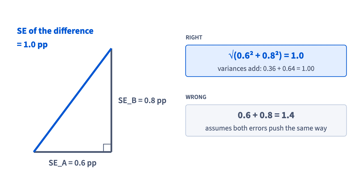
For the difference between two shares, Newcombe's interval reuses two Wilson intervals. Each group gets its own Wilson interval, and the distance from its estimate to an end of that interval is a one-sided width, w_A and w_B. The groups are independent, so the widths combine by Pythagoras: √(w_A² + w_B²).

With widths of 0.6 and 0.8 pp, the combined width is √(0.36 + 0.64) = 1.0 pp, not 1.4. Same shape, new inputs. Whenever you see a square root of a sum of squares, read it as "independent pieces combined".

How it fits together: Pythagoras gives straight-line distances between learners, the SE of a difference, the uncertainty of a chain of tasks and the Newcombe width, always for independent pieces. The next lesson divides by such spreads to put different numbers on one scale: z, CV, effect size and r.