Other curves and power

t-tests, chi-square tests and ANOVA look like three subjects. They are one idea with different tables.

Every test squeezes the data into one number, the statistic: roughly signal ÷ noise. Then it asks how far into the tail of its own curve that number lands. The point that leaves 5% beyond it is the critical value; a statistic past it counts as significant at 5%.

The curves differ, so the cut-offs do too: 1.96 for z, 2.101 for t with 18 degrees of freedom, 3.84 for chi-square with 1, 3.10 for F with (3, 20). You don't compute these; you read them from a table or a spreadsheet.

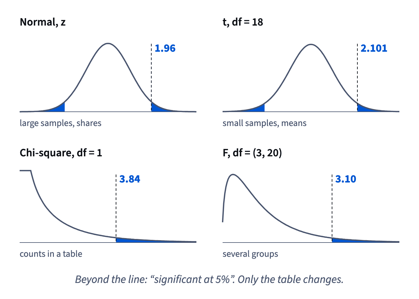
The classic slip is borrowing z's 1.96 for everything. A t of 2.05 from two groups of 10 clears 1.96 but not 2.101, so it is not significant at 5%.

The question you ask picks the statistic, and the statistic picks its curve.

• Comparing the means of two small groups, say 10 learners each: a t statistic, its curve set by n₁ + n₂ − 2 = 18 degrees of freedom, critical value 2.101.
• A table of counts, such as booked or not, with or without a reminder: chi-square, with (rows − 1)(columns − 1) = 1 degree of freedom for a 2×2 table, critical value 3.84.
• The means of several groups, say four groups of 6: F, with two degrees of freedom, (groups − 1, people − groups) = (3, 20), critical value 3.10.
• Shares in two large groups: z, critical value 1.96.

Each pairing is the same move: compute the statistic, find the critical value for its curve and degrees of freedom, compare.

Degrees of freedom (df) say roughly how much independent information is left after the statistic has used some of it. They choose which member of a curve family to read.

Each estimate made from the data uses one up. A t-test on two groups estimates two means, so df = n₁ + n₂ − 2: for 12 and 15 learners, 12 + 15 − 2 = 25. A table with r rows and c columns has (r − 1)(c − 1): once the row and column totals are fixed, only that many cells are free to vary. F for k groups and N people has two: (k − 1, N − k).

The count matters most for small samples. With few degrees of freedom the curve has heavier tails and a higher cut-off; with many, it settles down. Getting df wrong means reading the wrong row of the table.

The t curve looks like the normal curve with heavier tails. With a small sample, the noise itself is estimated from few people, so extreme statistics happen more often by chance. To keep the false-alarm rate at 5%, the cut-off moves out: 2.228 at 10 degrees of freedom, 2.101 at 18.

As the sample grows, the estimate of the noise steadies and the tails thin. At 30 degrees of freedom the cut-off is 2.042; at 100 it is about 1.98, almost z's 1.96. For large samples t and z give practically the same verdict.

So the t table matters for small groups, a pilot with a dozen learners per arm, and hardly at all for product tests with thousands of users. Using 1.96 on a small sample makes a test look more convincing than it is.

A chi-square test compares a table of observed counts with the counts you'd expect if the groups didn't differ. The first step is those expected counts.

If group made no difference, every group would share the overall rate. Klasna's goal-setting call: with it 105 of 300 bought, without it 125 of 500, overall 230 of 800 = 28.75%. So the 300 called learners would be expected to produce 300 × 0.2875 = 86.25 buyers.

Written as one rule: E = row total × column total ÷ grand total. For the call: 300 × 230 ÷ 800 = 86.25. For Club members who joined a speaking club in week one: 200 joined, 180 of all 800 members cancelled, so E = 200 × 180 ÷ 800 = 45 cancellations expected among the 200, against 30 observed.

Expected counts may have decimals; don't round them. They are averages under "no difference", not people.

With the expected counts in place, each cell adds its surprise: (O − E)² ÷ E, the squared gap between observed and expected, scaled by the expected count. The chi-square statistic is the sum over all cells: χ² = Σ(O − E)² ÷ E.

For Klasna's goal-setting call the four cells give 4.076 + 1.645 + 2.446 + 0.987 ≈ 9.15. With 1 degree of freedom the cut-off is 3.84, so the difference is significant.

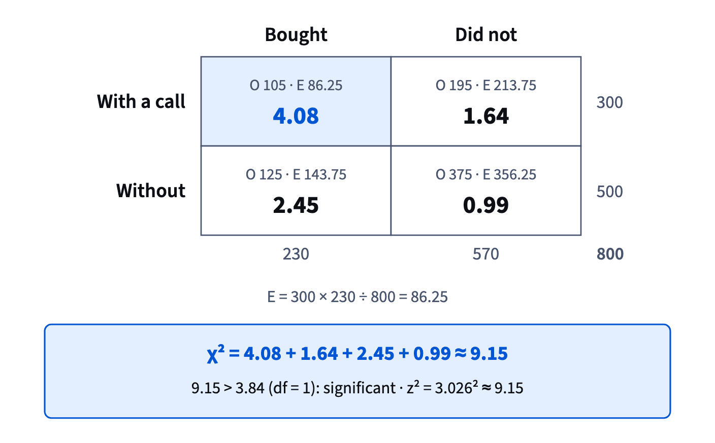
For a 2×2 table there is a shortcut: chi-square equals the square of the two-proportion z. The same data give z ≈ 3.026, and 3.026² ≈ 9.15. Even the cut-offs match: 1.96² = 3.84. So for two groups and a yes/no outcome the two tests are one test written two ways; a z of 2.5 means χ² = 6.25.

Chi-square earns its keep on bigger tables, such as three packages × two age groups, where a single z doesn't fit.

Power is the chance that a test catches an effect that is really there. Start from the shifted curve: if the true effect is δ and the difference is measured with standard error SE, the measured difference sits on average δ ÷ SE standard errors from zero. A two-tailed 5% test calls it significant when it lands past 1.96. So power ≈ P(Z > 1.96 − δ ÷ SE).

When δ ÷ SE = 2.8, power is P(Z > −0.84) = 80%, the usual target. A real 2 pp effect measured with SE = 0.8 pp gives δ ÷ SE = 2.5, 1.96 − 2.5 = −0.54, and P(Z > −0.54) = 70.5%.

The product-analytics course's paywall test, 1,700 users per variant, 4% against 5%: SE ≈ 0.0071, δ ÷ SE ≈ 1.41, power = P(Z > 0.55) ≈ 29%. Seven times in ten a real +1 pp lift would come out "not significant".

Power ≈ P(Z > 1.96 − δ ÷ SE) has three levers, and only two are yours.

• A smaller SE. More people, or a less noisy metric. Because SE shrinks with √n (from Square roots and √n), four times the users halves it. For the paywall test, 6,800 per variant instead of 1,700 takes δ ÷ SE from 1.41 to about 2.81 and power from 29% to about 80%.
• The cut-off. A stricter level, 1% instead of 5%, moves 1.96 out to 2.576 and lowers power; that is the price of fewer false alarms.
• The effect δ. It is what it is. Planning for a bigger effect than you expect only makes the power on paper look better.

Peeking or adding metrics doesn't help: they raise false alarms, not power.

How it fits together: every test compares a statistic with its curve's critical value; degrees of freedom pick the curve; chi-square sums observed-versus-expected gaps; power is the shifted curve's area past the cut-off. The next module is unit economics, starting with contribution margin and break-even.