e, ln, odds and the sigmoid

Growth questions often ask "how long?": how long until money doubles, until a metric hits a target. The unknown then sits in the exponent: aᵗ = b. The natural logarithm, ln, brings it down, because ln(aᵗ) = t × ln a. So t = ln b ÷ ln a.

Example: how long does money take to double at 25% a year? 1.25ᵗ = 2, so t = ln 2 ÷ ln 1.25 = 0.6931 ÷ 0.2231 ≈ 3.1 years. Check: 1.25³ ≈ 1.95, just short of 2.

ln is a calculator button and a spreadsheet function (=LN). For this ratio any logarithm works, as long as the top and the bottom use the same one.

Two habits help. Take ln of the growth factor (1.25), not of the rate (0.25): ln 0.25 is negative and gives nonsense. And check with a power: the t you found should make aᵗ close to b. Isolate the power first, as in Rearranging a formula: solve for what you need, then take ln.

e ≈ 2.718 is a constant like π, and it falls out of growth. Take 1 at 100% a year. Add the interest once and you get 2. Add it monthly and you get (1 + 1/12)¹² ≈ 2.613. Daily, (1 + 1/365)³⁶⁵ ≈ 2.715. Continuously, the limit of (1 + 1/n)ⁿ as n grows, you get e.

So eˣ is a growth factor: e^0.5 ≈ 1.65, e¹ ≈ 2.72, e⁰ = 1, e⁻¹ ≈ 0.37. And ln is the power of e that gives a number: ln(eˣ) = x, ln 1 = 0, ln e = 1. The two undo each other, like squaring and the square root.

Why it matters here: logistic models, continuous growth and many statistics formulas are written with e and ln. You never compute e by hand; you read eˣ as "a factor" and ln as "the power that makes this factor".

Landmarks: ln of a number above 1 is positive, ln of a number between 0 and 1 is negative, and ln 0 doesn't exist.

Odds compare yes with no: odds = p ÷ (1 − p), where p is the probability of yes and 1 − p the probability of no, the pair that p and 1 − p covers in module 7. If 20% of trial learners buy a package, the odds are 0.2 ÷ 0.8 = 0.25, "one to four": one buyer for every four who don't.

Landmarks: p = 0.5 gives odds of 1, "even"; p = 0.75 gives 3; p = 0.9 gives 9; p = 0.1 gives about 0.11. Odds run from 0 to infinity, and they grow fast as p nears 1.

Odds aren't a probability. "Odds of 3" is neither "300%" nor "30%": it says yes is three times as likely as no, which is p = 0.75.

Odds turn up wherever logistic models, bets and 2 × 2 tables do. Their advantage is that multiplying odds always gives valid odds, while multiplying a probability can push it past 1.

To turn odds back into a probability, divide them by one plus themselves: p = odds ÷ (1 + odds). Odds of 1.5 give 1.5 ÷ 2.5 = 0.6; odds of 0.25 give 0.25 ÷ 1.25 = 0.2. Check by going forward: 0.6 ÷ 0.4 = 1.5.

Odds are lopsided around 1. Everything below "even" is squeezed between 0 and 1, everything above spreads out to infinity. 0.25 and 4 are mirror images, one to four and four to one, yet they sit at very different distances from 1.

The logarithm fixes that. ln 0.25 ≈ −1.39 and ln 4 ≈ +1.39: the log-odds are symmetric around 0, which stands for p = 0.5. They run from minus to plus infinity, so a model can add contributions freely without ever producing an impossible probability.

That's why logistic models work on the log-odds scale, z = ln(odds), and convert back to a probability only at the end.

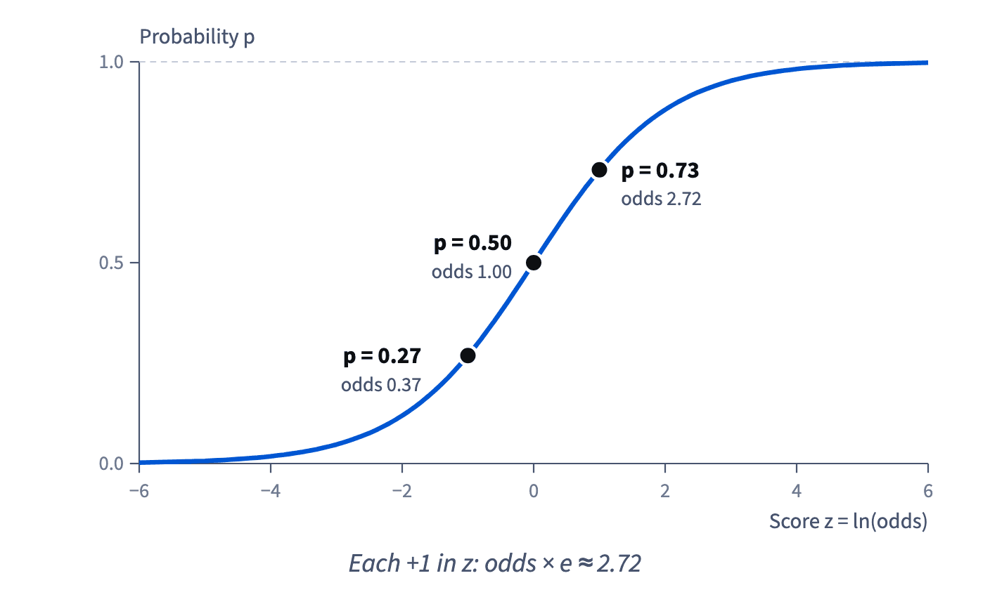
A logistic model adds up a score on the log-odds scale, for example z = −1.5 + 0.5 × lessons in the first week. The sigmoid turns any z into a probability between 0 and 1: p = 1 ÷ (1 + e⁻ᶻ).

Worked values for that model: 3 lessons give z = 0, so p = 1 ÷ (1 + 1) = 0.5. 5 lessons give z = 1, so p = 1 ÷ (1 + e⁻¹) = 1 ÷ 1.368 ≈ 0.73. 1 lesson gives z = −1 and p = 1 ÷ (1 + e) ≈ 0.27.

The curve is S-shaped: steep in the middle, flat at the ends. Near p = 0.5 a step in z moves the probability a lot; near 0 or 1 the same step barely moves it. It never reaches 0 or 1, however large z gets.

Order of operations matters, as in Order of operations, ratios and multiples: compute z first, then e⁻ᶻ, then 1 + e⁻ᶻ, then divide. Watch the minus: z = −1 puts e⁺¹ in the denominator.

In a logistic model a coefficient b adds to the log-odds. Adding inside ln is multiplying outside, so one more unit of that variable multiplies the odds by eᵇ. It does not add b to the probability.

Example: b = 0.5 per lesson in the first week means each extra lesson multiplies the odds of buying by e^0.5 ≈ 1.65. A whole step of 1 in z multiplies the odds by e ≈ 2.72: z = 0 is odds of 1, z = 1 is odds of 2.72.

What that does to the probability depends on the start. Take b = 0.4, a factor of e^0.4 ≈ 1.49. From p = 0.2 (odds 0.25) the odds become 0.37 and p ≈ 0.27; from p = 0.5 (odds 1), 1.49 and p ≈ 0.60; from p = 0.9 (odds 9), 13.4 and p ≈ 0.93.

So report "about 1.5 times the odds", and when you translate it into a probability, say from which starting point.

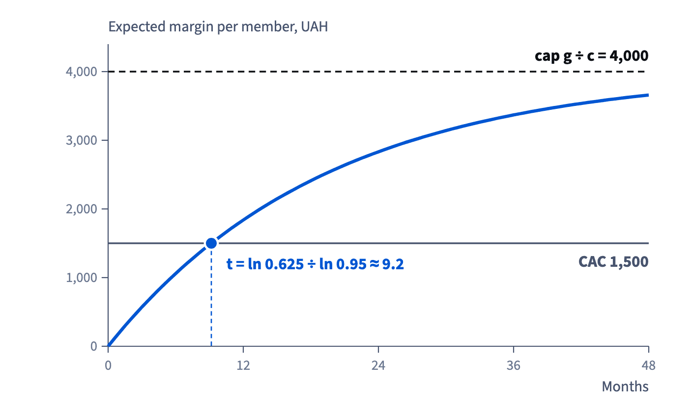
Combine the finite sum from Geometric series with ln. A member brings margin g a month and churn c thins the group, so after t months the expected margin is g × (1 − (1 − c)ᵗ) ÷ c. Payback is the t where this equals the acquisition cost, CAC.

Rearrange: (1 − c)ᵗ = 1 − CAC × c ÷ g. Take ln: t = ln(1 − CAC·c ÷ g) ÷ ln(1 − c).

Example: g = 200 UAH, c = 5%, CAC = 1,500. 1 − 1,500 × 0.05 ÷ 200 = 0.625; t = ln 0.625 ÷ ln 0.95 ≈ −0.470 ÷ −0.0513 ≈ 9.2 months.

The curve flattens towards the cap g ÷ c = 4,000, the LTV. If CAC is at or above the cap, the bracket is zero or negative, ln has no answer, and the member never pays back. Check the cap first.

How it fits together: ln brings exponents down, e builds growth factors, odds and the sigmoid link scores to probabilities, and payback with churn joins them. Module 7 turns to probability itself: complements, conditional probability, expected value and the normal curve.