Conditional probability and the 2×2 table

A conditional probability P(A | B), read "A given B", is the probability of A counted only among the cases where B is true. The condition shrinks the denominator: P(A | B) = P(A and B) ÷ P(B).

Klasna's churn model shows how far a condition can move a number. Last month 80 of 1,000 Club members cancelled: P(cancel) = 0.08. The model flagged 120 members, and 48 of them cancelled: P(cancel | flagged) = 48 ÷ 120 = 0.40. Among the 880 it didn't flag, 32 cancelled: P(cancel | not flagged) = 32 ÷ 880 ≈ 0.036.

Counts and shares give the same answer: 48 of 1,000 is 0.048, 120 of 1,000 is 0.12, and 0.048 ÷ 0.12 = 0.40.

Before computing, say the condition out loud: "among the flagged…", "among those not flagged…". Then divide by that group only, never by everyone.

Two yes/no questions about the same people make a 2×2 table: rows for one question, columns for the other, and four cells that add up to the total. For Klasna's churn model the rows are what the model said (flagged, not flagged) and the columns are what happened (cancelled, stayed).

The cells have names: true positives, flagged and cancelled (TP = 48); false positives or false alarms, flagged but stayed (FP = 72); false negatives or misses, not flagged but cancelled (FN = 32); and true negatives, not flagged and stayed (TN = 848).

You rarely get all four cells. Usually you know the total (1,000), a row total (120 flagged), a column total (80 cancelled) and one cell (48). The rest is subtraction: 120 − 48 = 72, 80 − 48 = 32, 1,000 − 48 − 72 − 32 = 848. Check that the cells add back to the total before computing anything from them.

Most numbers you take from a 2×2 table are conditional probabilities that keep one numerator and change the denominator.

• Precision = TP ÷ (TP + FP) reads the flagged row: of the people support calls, how many were about to cancel? 48 ÷ 120 = 0.40.
• Recall = TP ÷ (TP + FN) reads the cancelled column: of everyone who cancelled, how many did the model catch? 48 ÷ 80 = 0.60.
• Accuracy = (TP + TN) ÷ all counts every correct cell: (48 + 848) ÷ 1,000 = 0.896.
• The base rate ignores the model: 80 ÷ 1,000 = 0.08.

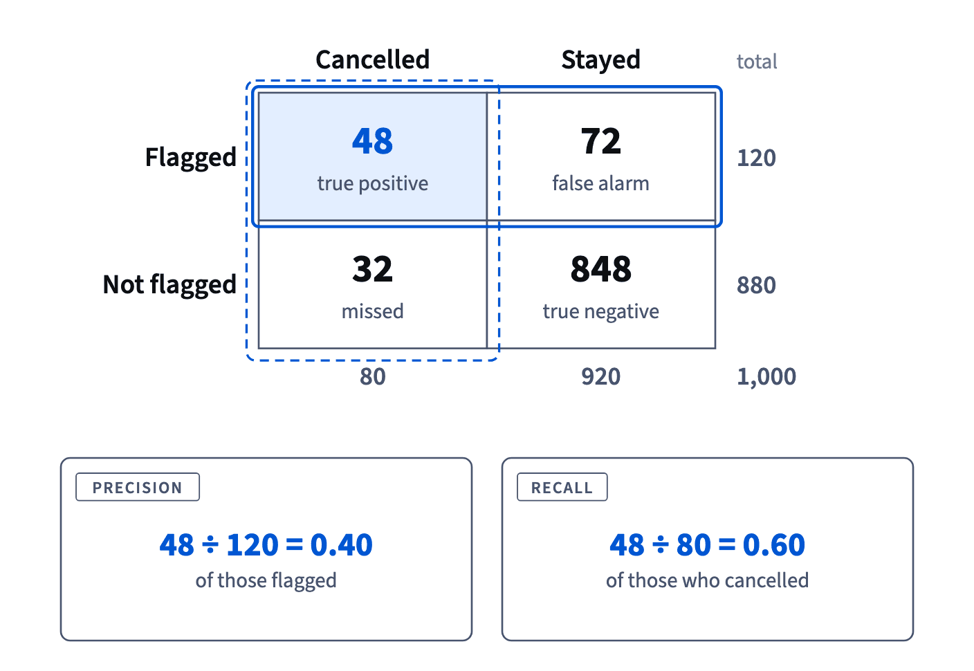
To tell them apart, ask what the number divides by. Precision is a share of the flags; recall is a share of the real cases. The same 48 sits on top of both, which is exactly why reports swap them so easily.

Accuracy is the share of all cases a model got right. It sounds like the natural score, but when the event is rare it is dominated by the easy "no"s.

In Klasna Club only 80 of 1,000 members cancel in a month. A model that flags nobody is right about all 920 who stay: accuracy 0.92. The real churn model, which catches 48 cancellations, scores 0.896, lower than doing nothing. Accuracy rewards the lazy model because true negatives fill almost the whole table.

So when a team acts on a flag, accuracy is the wrong headline. Ask two questions instead: how many of our actions are wasted (precision), and how many real cases slip past (recall)? Compare any accuracy with the base rate as well: a model is useful only if it beats "always say no", which here already scores 1 − 0.08 = 0.92.

A churn model doesn't just say yes or no: it scores every member, and the team picks a threshold. Flag more people and you catch more of the real cases, but more of the flags are false alarms. Flag fewer and the opposite happens.

The first model flags 120 members and catches 48 of the 80 who cancel: recall 0.60, precision 0.40. A second model flags 300 and catches 72: recall 72 ÷ 80 = 0.90, precision 72 ÷ 300 = 0.24. Neither is simply better. The second reaches more members who are about to leave, and wastes more calls doing it.

Which matters more depends on the cost of each mistake. If a call is cheap and losing a member is expensive, high recall is worth many wasted calls. If each action costs a lot, a discount for example, precision matters more. Report both numbers and say which trade-off you chose.

P(A | B) and P(B | A) share a numerator, the cases where both happen, but divide by different groups, so they are usually different numbers. P(cancel | flagged) = 48 ÷ 120 = 0.40, while P(flagged | cancel) = 48 ÷ 80 = 0.60. Swapping the condition is the most common probability mistake in reports.

Test results are where it bites. A p-value is P(data this extreme | no real effect), not P(no real effect | data). Some test reports show the other direction, "probability that B beats A: 59%", which is P(B better | data) = 0.59. Read it literally: given what we saw, B is better slightly more often than a coin toss would suggest. It doesn't say B converts 59% better, and it doesn't say 59% of users preferred B.

Before quoting a conditional probability, put both sides into words: "the share of X among Y". If the sentence changes meaning when you swap X and Y, so does the number.

A 2×2 table can also compare two groups: the rows are the groups, the columns the outcome. The simplest comparison is the relative risk: the outcome's probability in one group divided by its probability in the other, RR = p₁ ÷ p₂.

Klasna gave some trial learners a short goal-setting call: 105 of 300 bought (0.35), against 125 of 500 without a call (0.25). RR = 0.35 ÷ 0.25 = 1.40: with the call, buying was 1.4 times as likely. An RR of 1 means no difference; below 1, the outcome is less likely in the first group.

Two habits help. Compute each group's probability inside its own row, never over the grand total. And say which group is on top: 1.40 one way is 0.71 the other way (0.25 ÷ 0.35). "Buying was 1.4 times as likely" and "the call raised buying by 40%" say the same thing; "by 140%" does not.

Odds compare yes with no inside one group: odds = p ÷ (1 − p), the probability divided by its complement, as in e, ln, odds and the sigmoid. The odds ratio divides one group's odds by the other's: OR = (a ÷ b) ÷ (c ÷ d) = ad ÷ bc, where a and b are the yes and no counts of the first row, c and d of the second.

For the goal-setting call: odds 105 ÷ 195 = 0.538 with the call and 125 ÷ 375 = 0.333 without, so OR ≈ 1.62, while the relative risk was 1.40. The odds ratio always sits further from 1, because odds stretch faster than probabilities as p grows. For rare outcomes, 2% against 1%, the two nearly agree.

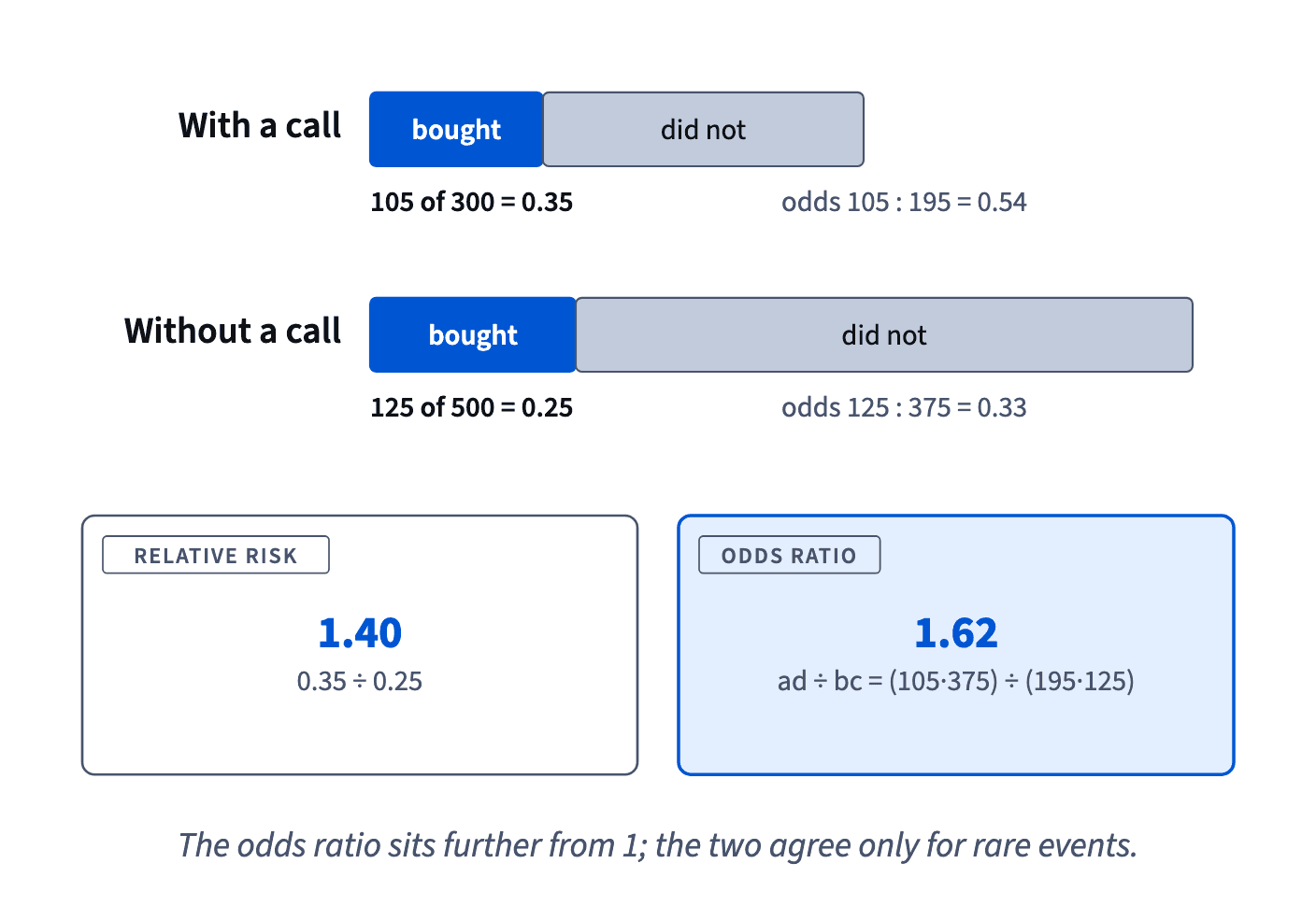
Logistic regression reports odds ratios, so read 1.62 as "the odds are 1.62 times as high", never as "1.62 times as likely".

How it fits together: a condition shrinks the denominator; the 2×2 table holds every count, and each metric picks its own row, column or total. The next lesson weighs outcomes by how likely they are: expected value.