

Theory
Sample vs population and the normal distribution
Sample vs population: why we study samples to learn about all users, why the bell-shaped normal distribution shows up everywhere, and how the central limit theorem ties them together.
~11 min read · 11 exercises · 250 points
Before you start
From 500 orders to every customer
A new module at CatChow: soon the product team will compare groups and read A/B tests. First, Alex, the team's analyst, wants everyone to agree on what is being measured. You've already pulled last month's 500 orders into a sheet, but what can they say about every customer who has ever bought, or ever will?
This lesson covers samples and populations, the bell-shaped normal distribution, and the theorem that links the two.
Sample, population, parameter, statistic
Almost every number a product team looks at comes from a sample: the part of the users or orders you actually measured. What you really care about is the population: everyone the decision is about, including customers who haven't arrived yet. You can almost never measure the population, so you measure a sample and generalise.

The same split applies to numbers:
- a parameter describes the population, for example the true average order value of every CatChow customer. It exists, but you don't know it;
- a statistic is computed from a sample, for example the average of the 500 orders you pulled. You know it exactly, and you use it to estimate the parameter.
A quick test: ask "was this number calculated from data I have?" If yes, it's a statistic. A survey average from 10% of customers is a statistic even when the plan is to describe all customers with it. Describing everyone is the goal; it doesn't turn the number into a parameter.
- Do“Our 500 orders average $45, so we estimate the average for all customers is around $45.”
A statistic used as an estimate of the parameter.
- Don't“The average order of all our customers is $45.”
Presents a sample number as if it were the parameter itself.
Four words the rest of the course relies on
Statistics pairs these words up, and it helps to learn them as two pairs:
- population and parameter: the whole group and the true number about it. Usually unknown;
- sample and statistic: the part you measured and the number you calculated from it. Always known.
You'll also see different symbols for the two sides. Population values get Greek letters: μ (mu) for the mean and σ (sigma) for the standard deviation. Sample values get Latin ones: x̄ (x-bar) for the sample mean and s for the sample standard deviation. When a formula uses μ and σ, it assumes you know the whole population; when it uses x̄ and s, it works from data you actually have.
Why fuss over vocabulary? Because every test later in the course asks the same question: given this statistic, what can we say about the parameter? If the two get mixed up, a report quietly claims more certainty than the data can give.
- Dox̄ = $45 from 500 orders (statistic); μ = the unknown average of all orders (parameter).
- Don't“μ = $45” written next to a 500-order sample.
The Greek letter claims you measured everyone.
The normal curve and the 68-95-99.7 rule
A normal distribution is the symmetric bell curve. Values pile up around the middle and thin out evenly on both sides, and the mean, median and mode all sit at the centre. It tends to appear when a value is the sum of many small, independent nudges.
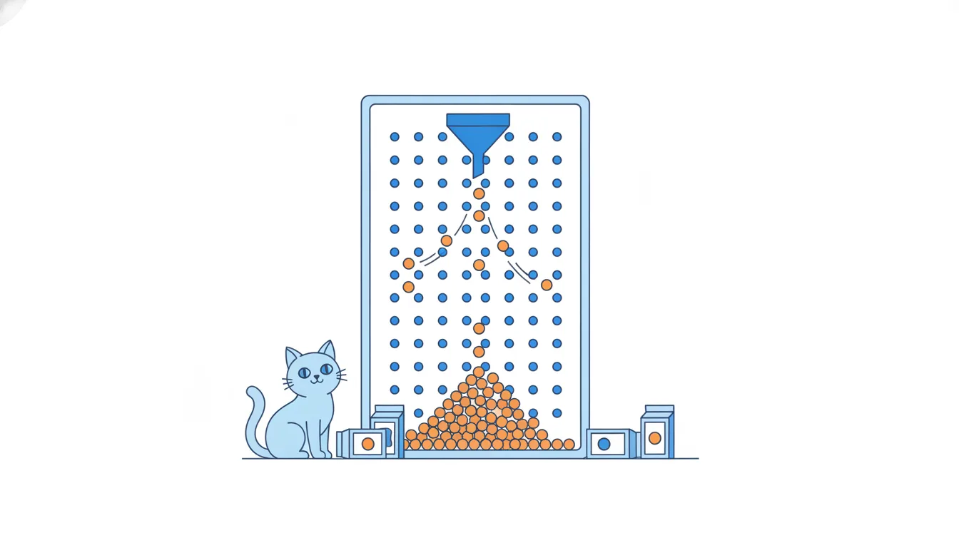
Two numbers describe it completely: the mean (where the centre is) and the standard deviation (how wide the bell is). Once you know them, the empirical rule tells you where most values fall:
- about 68% within 1 standard deviation of the mean;
- about 95% within 2;
- about 99.7% within 3.
Chart data
| z-score | Density |
|---|---|
| -3 | 0.004 |
| -2.5 | 0.018 |
| -2 | 0.054 |
| -1.5 | 0.13 |
| -1 | 0.242 |
Show 8 more rows
| -0.5 | 0.352 |
| 0 | 0.399 |
| 0.5 | 0.352 |
| 1 | 0.242 |
| 1.5 | 0.13 |
| 2 | 0.054 |
| 2.5 | 0.018 |
| 3 | 0.004 |
With a mean of $50 and a standard deviation of $12, that means about 68% of orders between $38 and $62, about 95% between $26 and $74, and almost all between $14 and $86.
The rule only works for data that is roughly bell-shaped. Real order values often have a long tail of big orders, so check the histogram before you lean on it.
- DoMean $50, SD $12: about 95% of orders fall between $26 and $74 (50 ± 2 × 12).
- Don'tApplying 68-95-99.7 to order values with a long tail of bulk orders without checking the shape.
The rule describes a bell, not every dataset.
Where sampling bias comes from
A sample is useful only if it looks like the population in the ways that matter. Sampling bias appears when the chance of being picked is linked to the thing you measure. Then a bigger sample doesn't help: you just get a more precise wrong answer.
Two common ways it sneaks in:
- the channel filters people. A survey sent only as an app push reaches app users and misses everyone who orders on the website. If app users are happier or more loyal, the average is off;
- the moment filters people. Surveying people right after they contacted support oversamples the ones who had a problem.
Methods that break the link are fine: a random draw from the full customer list, or taking every 20th name from a list sorted by something unrelated, like the alphabet.
Before trusting a number, ask: who could not have ended up in this sample, and might they answer differently? If the answer is yes, the result describes a subgroup, not all customers.
- DoDraw 2,000 customers at random from the full database and email all of them.
Everyone has the same chance of being asked.
- Don'tPut the satisfaction survey only on the “Order delivered” screen of the app.
Website shoppers and failed deliveries never see it.
z-scores: distance from the mean in standard deviations
A z-score tells you how many standard deviations a value sits from the mean:
z = (x − μ) / σ
Formula: z-score: subtract the population mean μ from the value x, then divide by the population standard deviation σ. · shown above
First subtract the mean, then divide by the standard deviation. The order matters: dividing first gives nonsense.
With μ = $50 and σ = $12, an order of $74 has z = (74 − 50) / 12 = 24 / 12 = 2.0. An order of $38 has z = (38 − 50) / 12 = −1.0: one standard deviation below the mean. A z-score of 0 is exactly average.
Why bother? Because z-scores put very different measures on one scale. A $74 order and a 9-minute session can't be compared directly, but "2 standard deviations above normal" can. Combined with the empirical rule, a z-score also tells you how unusual a value is in a roughly normal distribution: beyond ±2 is rare (about 5% of values in total), beyond ±3 is very rare.
Keep in mind that this reading assumes a bell shape; in a skewed distribution, z = 2 is less unusual on the long side.
- Do(74 − 50) / 12 = 2.0
Subtract the mean first, then divide.
- Don't74 / 12 ≈ 6.17
Forgets the mean, so the result is not a distance from anything.
Sampling distributions and the central limit theorem
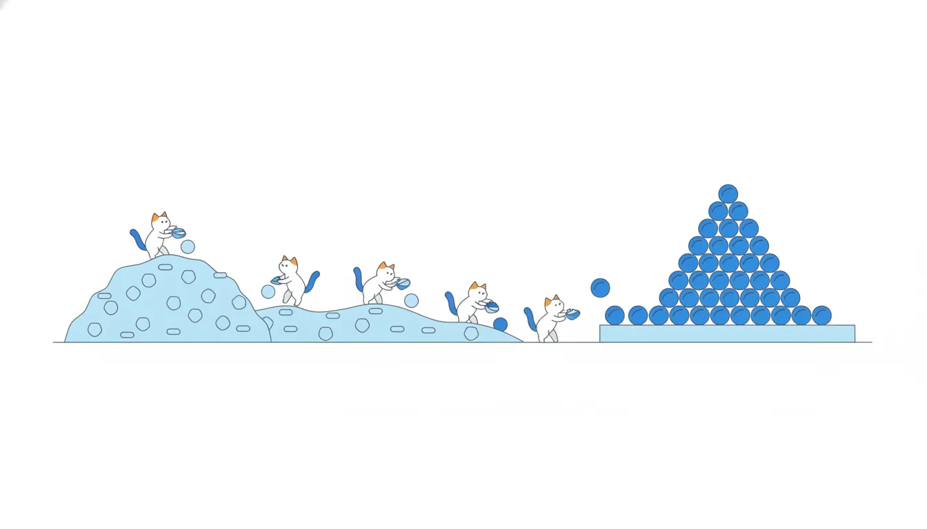
Imagine drawing many different samples of 40 orders and computing the mean of each. The means won't be identical: each sample catches slightly different customers. The spread of all those possible sample means is the sampling distribution of the mean.
The central limit theorem (CLT) says something surprising about its shape: as the sample size n grows, the sampling distribution of the mean gets closer and closer to normal, whatever the shape of the original data. Order values can be heavily skewed, with a long tail of bulk orders, and the means of samples of them will still form a near-bell.
Two things the CLT does not say:
- it doesn't make the raw data normal. Individual orders stay skewed no matter how many you collect;
- it doesn't name one magic n. Mildly skewed data may need a few dozen observations per sample; data with extreme outliers needs many more.
This is why tests built on the normal curve work on business metrics that are far from normal themselves.
- Do“Order values are skewed, but the mean of 200 orders is close to normally distributed, so a normal-based test is reasonable.”
- Don't“We collected 5,000 orders, so by the CLT the order values are now normal.”
The CLT is about sample means, not the raw values.
Standard error is not standard deviation
Two spreads, two questions:
- the standard deviation (s) says how much individual values differ from each other. One order is $20, another $70;
- the standard error (SE) says how much the sample mean would move if you repeated the sampling. It's the width of the sampling distribution.
You estimate it from one sample:
SE = s / √n
Formula: Standard error of the mean: the sample standard deviation s, divided by the square root of the sample size n. · shown above
With s = $18 and n = 36 orders: SE = 18 / √36 = 18 / 6 = $3. Individual orders swing by around $18, but the average of 36 of them is pinned down to within a few dollars.
The standard error shrinks as n grows, because averaging cancels out random highs and lows. The standard deviation doesn't shrink with more data: it describes the customers, not your uncertainty.
A common slip is to forget the square root and divide by n itself: 18 / 36 = 0.5 understates the uncertainty six times over. Another is to report the SE where the spread of individual values is needed, which makes the data look far more uniform than it is.
- DoSE = 18 / √36 = 18 / 6 = 3
- Don'tSE = 18 / 36 = 0.5
Divides by n instead of √n.
The square-root law: why precision gets expensive
Because the standard error divides by √n rather than n, precision grows slowly. To halve the standard error you need four times the data, not twice.
Formula: Standard error of the mean: the sample standard deviation s, divided by the square root of the sample size n. · shown above
With s = $18:
- n = 36 gives SE = 18 / 6 = $3.00;
- n = 144 gives SE = 18 / 12 = $1.50;
- n = 576 gives SE = 18 / 24 = $0.75.
Each halving costs four times the previous sample. Doubling from 36 to 72 orders only takes the SE from $3.00 to about $2.12.
To find the sample you need for a target SE, turn the formula around: √n = s / SE, then square it. For a target of $1.50: √n = 18 / 1.5 = 12, so n = 144.
This matters whenever someone asks for "just a bigger sample". The first few hundred observations buy a lot of precision; after that, each extra digit of precision costs weeks of traffic. It's often cheaper to accept a slightly wider interval, or to reduce noise in the metric, than to keep collecting.
- DoTarget SE $1.50: √n = 18 / 1.5 = 12, n = 144 (4 × 36).
- Don't“Twice the orders, half the error”: n = 72.
With 72 orders the SE is still about $2.12.
Reading a standard error in a report
A standard error answers one question: how far is the sample mean likely to be from the population mean? It doesn't describe customers, it describes your uncertainty about the average.
A handy rough reading: the population mean is probably within about 2 standard errors of the sample mean. With a sample mean of $45 and SE = $3, that's 45 ± 6, so roughly $39 to $51 for the average order of all customers. Later lessons make this interval precise; for now, "mean ± 2 SE" is a good sanity check.
The classic misreading is to apply that interval to individual orders. With s = $18, single orders range far wider: if they were roughly normal, about 95% would fall within 45 ± 36, from $9 to $81. The $39–$51 band is about the average, not about any one customer.
When you write a result, say which spread you mean: "orders vary by about $18 (SD)" or "the average is known to within about $6 (2 SE)".
- Do“Average order $45; the true average is probably between about $39 and $51.”
- Don't“Most customers spend between $39 and $51.”
Uses the SE interval to describe individual customers.
Ready to practise?
Answer the lesson's exercises and earn 250 points the first time you finish it.
Start the exercises