

Theory
Paired t-test: before and after
Comparing the same users before and after a change with a paired t-test or the Wilcoxon signed-rank test.
~11 min read · 11 exercises · 250 points
Before you start
Did the loyalty program work?
CatChow launched a loyalty program last month, and Marketing has brought the product team a question: did it really raise monthly spend, or would spend have drifted up anyway? This time the data follows the same eight customers before and after the launch.
That changes which test fits. In this lesson you'll compare before and after with a paired t-test and see why treating the same people as two separate groups throws information away.
Paired samples: each customer is their own baseline
Two samples are paired (related) when each value in one has a natural partner in the other: usually the same customer measured twice, before and after a change. Samples are independent when the two groups are different people, as in an A/B test.
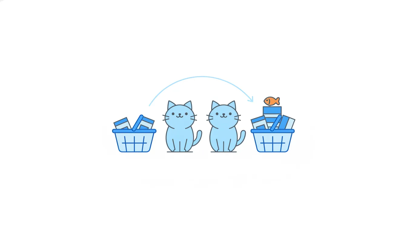
The design decides the test. For the loyalty program, CatChow tracked the same 8 customers' monthly spend before and after. Those customers differ a lot from each other: one spends $29 a month, another $60. That spread is real, but it has nothing to do with the program.
An independent-samples t-test treats "before" and "after" as two unrelated groups, so all that between-customer spread lands in its noise term. A paired t-test works on each customer's own change instead. Subtracting before from after removes their personal level and leaves only how much they moved.
The result: much less noise and much more power from the same data. The only requirement is that the pairing is real: the same people, or deliberately matched ones.
- DoSame 8 customers before and after → one column of differences → paired t-test.
- Don'tSame 8 customers, but compare the before average with the after average as two groups.
Throws the pairing away and buries the effect in between-customer noise.
What counts as a pair
A paired test subtracts one value from its partner, so every value needs a partner that belongs with it. Typical pairs in product work:
- the same user, twice: spend before and after a loyalty program, task time on the old and new checkout;
- the same user, two conditions: one person rates both versions of a page;
- deliberately matched units: two stores matched on size and city, one gets the change.
What isn't a pair:
- this month's buyers vs last month's buyers. Some overlap, but many people differ, and there's no one-to-one link;
- two A/B groups. Users are randomly split, so each person appears only once.
If you can't write the data as one row per unit with a "before" and an "after" column, it isn't paired.
Using a paired test on unpaired data is not a small error: the subtraction pairs up random strangers, and the result is meaningless. Using an independent test on paired data is valid but wasteful: you lose power you already paid for.
- DoOne row per customer: U1 42 → 47, U2 38 → 40, … → paired.
- Don'tPair September’s 200 buyers with October’s 200 buyers in list order.
Different people in arbitrary order are not pairs.
Step one: the mean difference
A paired analysis starts by collapsing each pair into one number: the difference d = after − before.
For the 8 loyalty customers:
- U1 47 − 42 = 5, U2 40 − 38 = 2, U3 59 − 51 = 8, U4 30 − 29 = 1;
- U5 66 − 60 = 6, U6 37 − 33 = 4, U7 50 − 47 = 3, U8 62 − 55 = 7.
Chart data
| Customer | After − before |
|---|---|
| U1 | 5 |
| U2 | 2 |
| U3 | 8 |
| U4 | 1 |
| U5 | 6 |
Show 3 more rows
| U6 | 4 |
| U7 | 3 |
| U8 | 7 |
The mean difference is d̄ = (5 + 2 + 8 + 1 + 6 + 4 + 3 + 7) / 8 = 36 / 8 = $4.50.
From here on, the two original columns are gone. The question becomes a one-sample question: is the mean of these 8 differences different from zero?
Two habits keep this clean. First, fix the direction (after minus before) and keep it for every customer; mixing directions flips signs and cancels real changes. Second, look at the differences before testing anything. Here all 8 are positive, which already tells you a lot. One huge difference among small ones would warn you about an outlier.
The mean difference also equals the difference of the two means (48.875 − 44.375 = 4.5), but only the paired view shows how consistent the change is.
- Dod̄ = 36 / 8 = $4.50
- Don'td̄ = 36 / 7 ≈ $5.14
n − 1 belongs in the variance, not in the mean.
Step two: the standard error of the differences
Next you need to know how much the mean difference would wobble from sample to sample. That's the standard error, computed from the differences alone:
SE = s_d / √n
where s_d is the standard deviation of the differences and n is the number of pairs.
For the 8 customers: the squared deviations of the differences from 4.5 add up to 42. Divide by n − 1 = 7 to get a variance of 6, so s_d = √6 ≈ 2.449. Then SE = 2.449 / √8 = 2.449 / 2.828 ≈ $0.87.
Compare that with the spread of the raw spend: before and after, customers vary with a standard deviation of roughly $11–$13. The differences vary by only about $2.45, because each customer's personal level has been subtracted out. That's where the paired test gets its power.
The slip to avoid: using the standard deviation of the raw before or after values instead of s_d. It brings the between-customer noise straight back in and makes the SE several times too big.
- DoSE = 2.449 / √8 ≈ 0.87
- Don'tSE = 10.8 / √8 ≈ 3.83 (SD of the “before” spend)
Uses the raw spread instead of the spread of the differences.
Step three: t, degrees of freedom and the decision
The paired t-statistic measures the mean difference in standard errors:
t = d̄ / (s_d / √n) = 4.5 / 0.866 ≈ 5.20
Formula: The paired t-test: mean difference divided by the standard error of the difference (SD of differences over the square root of n pairs). · shown above
The degrees of freedom count pairs, not values: df = n − 1 = 8 − 1 = 7. The 8 customers produced 16 numbers, but only 8 independent differences.
For a two-sided test at α = 0.05 with df = 7, the critical value is about 2.365. Our t is more than twice that, and the p-value is about 0.001. If the program truly changed nothing, a mean difference this large relative to its noise would be very rare.
That's significant evidence that spend rose, by about $4.50 per customer per month. It isn't yet evidence that the loyalty program caused it: without a control group, a seasonal rise would look exactly the same.
Two slips to avoid: using df = 14 (n1 + n2 − 2, the independent-samples formula), which uses a slightly lower critical value of about 2.145, and dividing by s_d instead of the SE (4.5 / 2.449 ≈ 1.84), which forgets the √n.
- Dot = 4.5 / 0.866 ≈ 5.20, df = 7, > 2.365
- Don'tt = 4.5 / 2.449 ≈ 1.84, “not significant”
Divides by the SD of the differences instead of their standard error.
Same data, two tests, very different answers
Run both tests on the loyalty data and the contrast is striking:
- independent-samples t-test: before mean $44.38, after mean $48.88. The customers' spend varies with a standard deviation of about $11–$13, so a $4.50 gap is small against that noise: t ≈ 0.76, p ≈ 0.46;
- paired t-test: the 8 differences range from +1 to +8, with a standard deviation of only $2.45: t ≈ 5.20, p ≈ 0.001.
Same numbers, same mean change, opposite conclusions. The difference is entirely in the noise term. The independent test counts the gap between a $29 customer and a $60 customer as noise, even though it has nothing to do with the program. The paired test subtracts it away.
This is why the design, not the result you prefer, picks the test. Measured the same people twice? Paired. Two separate groups? Independent. Running both and reporting the one you like is a form of p-hacking.
It also shows why a non-significant independent test on paired data says almost nothing: it was the wrong tool, not evidence of no effect.
- Do“Same 8 customers, so paired: t(7) ≈ 5.20, p ≈ 0.001.”
- Don't“We tried both tests and report the significant one.”
The design chooses the test before you see any p-value.
Four tools for paired data
Paired data have their own small toolbox:
- paired (related) samples: measurements that come in matched pairs, typically the same units measured twice. This is the design, not a test;
- paired t-test (Student's t-test for related samples): tests whether the mean of the differences is zero, t = d̄ / (s_d / √n), with n − 1 degrees of freedom. For the loyalty data, t ≈ 5.20 with df = 7, well beyond the critical 2.365, so p ≈ 0.001;
- sign test: counts how many differences are positive and how many negative, ignoring size;
- Wilcoxon signed-rank test: ranks the absolute differences and compares the rank sums of the positive and negative ones.
The t-test is the parametric option: most powerful when the differences are roughly normal. The other two are non-parametric fallbacks that trade a little power for fewer assumptions.
And one caveat that no test fixes: before/after data without a control group can't separate the program from everything else that changed over the same month, such as a season or a price change.
- Do“Paired t-test: t(7) = 5.20, p ≈ 0.001. No control group, so seasonality is a caveat.”
- Don't“The paired test proves the loyalty program caused the rise.”
It shows the change is real, not what caused it.
The sign test: counting pluses and minuses
The sign test is the simplest test for paired data. It throws away the size of each difference and keeps only its direction.
The logic: if the change did nothing, each customer's difference is as likely to be positive as negative, like a fair coin. So the number of pluses follows a coin-flip distribution, and you ask how unusual the observed count is.
For the loyalty data, all 8 differences are positive. The chance of 8 heads in 8 fair flips is 0.5⁸ = 1 / 256 ≈ 0.39%. A two-sided test also counts "all negative", so p ≈ 0.78%. Significant at 5%.
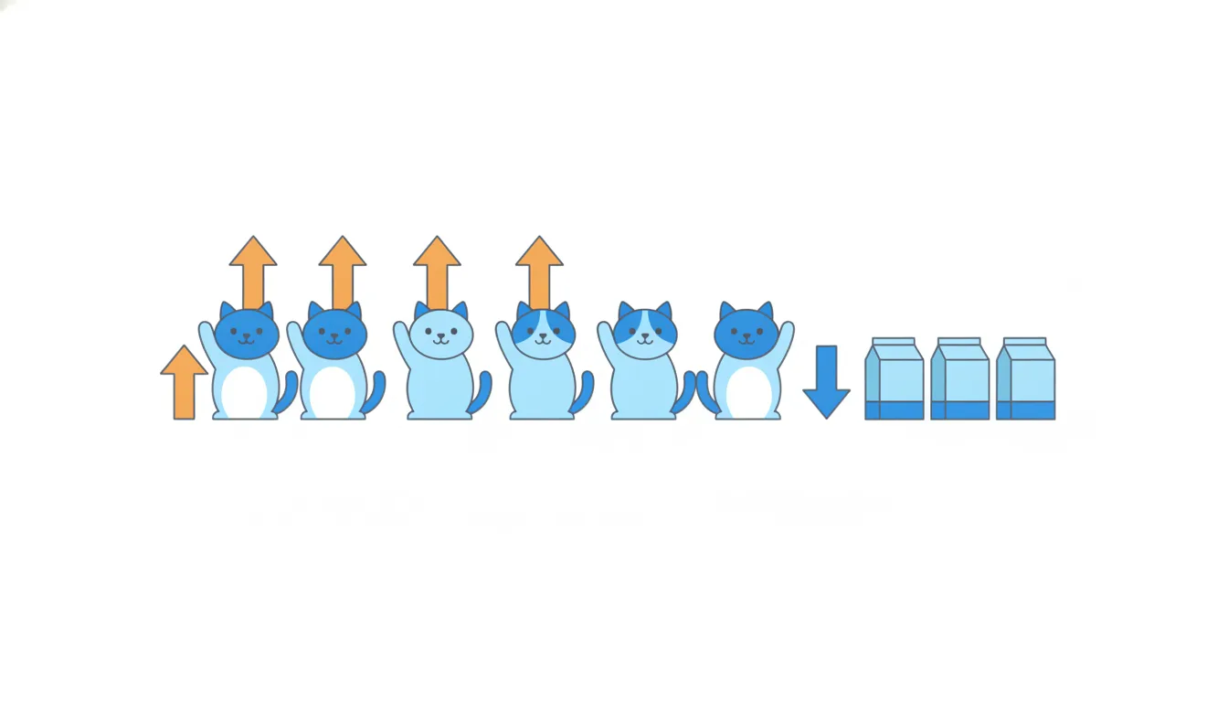
Differences of exactly zero carry no direction and are usually dropped, which reduces n.
When to use it: when only the direction is trustworthy, or when one or two extreme differences would dominate any test that uses sizes. With differences of +1, +1, +2, 0, +1 and +9, the +9 doesn't inflate anything here: it's just one more plus.
The price is power. With few pairs, the sign test needs nearly unanimous results; with 5 pairs, even 5 out of 5 gives a two-sided p of 0.0625.
- Do0.5⁸ = 1 / 256 ≈ 0.39% (one-sided)
- Don't0.5 × 8 = 4 → “50% chance”
Independent chances multiply; they don’t add.
Choosing between the paired t-test, Wilcoxon and the sign test
All three tests answer "did the values move?" from the same column of differences. They differ in how much of each difference they use.
- Paired t-test: uses the exact size of every difference. Most powerful, but it assumes the differences are roughly normal. With n − 1 degrees of freedom (7 for 8 pairs).
- Wilcoxon signed-rank test: uses the ranks of the absolute differences plus their signs. One extreme difference becomes just "the largest rank", so it's much safer with skew or outliers and loses little power.
- Sign test: uses only the direction, plus or minus. Very robust, and the least powerful.
A practical order: look at the differences first. Roughly symmetric, no wild values: paired t-test. A few extreme differences or a tiny sample: Wilcoxon. Only the direction is trustworthy (ratings that may not be comparable in size): sign test.
Whichever you use, pairing itself is what buys most of the power. It typically lets you detect the same effect with fewer people than two independent groups would need.
- DoDifferences +1, +1, +2, 0, +1, +9 with n = 6: Wilcoxon or sign test, not a t-test on the raw scores.
- Don't“The sign test is safest, so let’s always use it.”
Safety costs power; on clean data it throws information away.
Ready to practise?
Answer the lesson's exercises and earn 250 points the first time you finish it.
Start the exercises