Course recap: choosing the right test

Almost every method in this course is chosen by answering two questions.

1. What am I comparing? One variable's typical value, two groups, three or more groups, a relationship between variables, or groups nobody has defined yet.
2. Does the data meet the assumptions of a parametric test? A parametric test, like the t-test or ANOVA, compares means and relies on roughly normal data (or a large sample), no extreme outliers and a decent sample size. If that fails, use its non-parametric twin, which works on ranks instead of raw values.

For two independent groups:

• roughly normal data, decent n → Student's t-test (or Welch's t-test if the spreads differ);
• skewed data, small samples or extreme outliers → Mann-Whitney U test.

Time-on-page for 15 users per variant, heavily skewed with a couple of extreme values, is a textbook case for Mann-Whitney: two extreme sessions could swing both means, while ranks only care about order.

The cost of the non-parametric route is a little power when the data actually is normal, which is why it isn't the default for everything.

Before choosing a test for two sets of numbers, ask: are these different people, or the same people measured twice?

• Independent samples: different users in each group, as in an A/B test where each visitor sees only one variant. Use the t-test for independent samples or Mann-Whitney.
• Paired (related) samples: the same users measured before and after a change, or the same stores this month and last month. Each value has a natural partner.

For paired data, work with the differences within each pair:

• differences roughly normal → paired t-test (Student's t-test for paired samples);
• differences skewed or with outliers → Wilcoxon signed-rank test.

Why it matters: people differ a lot from each other, but much less from themselves. A paired test removes the person-to-person variation and compares each user only with their own earlier score, so it can detect a smaller change with the same 40 users. Treating paired data as independent throws that advantage away.

The same logic extends to three or more measurements of the same people: repeated-measures ANOVA, or the Friedman test for skewed data.

Whatever test you run, the estimate itself needs a sense of precision. The margin of error says how far the true value could plausibly be from your estimate. For a 95% confidence level it is about

margin of error ≈ 1.96 × SE

where SE is the standard error of the estimate: how much it would wobble from sample to sample.

If CatChow's conversion estimate has a standard error of 1.2 percentage points:

1.96 × 1.2 = 2.352 ≈ 2.35 percentage points.

Where does 1.96 come from? In a normal distribution, 95% of values lie within 1.96 standard deviations of the mean. The rough "2 standard errors" rule of thumb is the same idea, rounded.

Two slips to avoid:

• using the standard deviation of individual values instead of the standard error. The SD describes how individual users vary; the SE describes how the estimate varies, and is much smaller;
• forgetting the units. For a rate, the margin is in percentage points, not percent of the rate: ±2.35 points around 12% means 9.65% to 14.35%, not 12% ± 2.35% of 12%.

A confidence interval (CI) is the estimate with its margin of error on both sides:

CI = estimate ± margin of error

With a conversion estimate of 12.0% and a margin of 2.35 percentage points:

• lower bound: 12.0 − 2.35 = 9.65%;
• upper bound: 12.0 + 2.35 = 14.35%.

How to read it: if you repeated the same study many times, about 95% of intervals built this way would contain the true conversion rate. In practice, treat 9.65–14.35% as the range of values the data is compatible with. It is not a range where 95% of individual users fall, and it doesn't make every value inside equally likely: values near 12% are better supported than values near the edges.

Why report an interval rather than a bare p-value? It shows both the effect and its uncertainty in the metric's own units. An interval for a lift that runs from +0.1 to +4 points says "probably positive, size very uncertain"; one from +1.8 to +2.2 says "clearly positive and well measured".

The common slips: subtracting the margin twice, or adding a margin in percent of the rate to a rate in percentage points.

When the question is about how variables relate rather than how groups differ, the method depends on what you want to do and on what kind of outcome you have.

• How do two metrics move together? → correlation: Pearson's r for roughly linear, symmetric data; Spearman's ρ for skewed data, outliers or ranks. It describes; it doesn't predict.
• Predict a number from one or more predictors? → linear regression: simple with one predictor, multiple with several. Orders from ad spend, revenue from price and season.
• Predict a yes/no outcome? → logistic regression: it models the probability of "yes", always between 0 and 1. Will this customer churn, will this visitor buy.
• Assign new cases to known groups? → classification, of which logistic regression with a threshold is one example.

The outcome type is the quick filter: a continuous number points to linear regression, a yes/no to logistic. Using a straight line for churn gives "probabilities" like 1.3; using logistic regression for revenue makes no sense.

And for all of them: a relationship in past data isn't proof of cause. If the decision depends on cause, plan an experiment.

Some questions have no target variable: nobody is predicting churn or comparing variants, you just want to see structure. Two methods cover this, and the difference is what you group.

• Grouping observations (customers, stores, sessions) → cluster analysis. Customers with similar spend and order frequency end up in the same segment.
  • Don't know how many groups → hierarchical clustering, then cut the dendrogram where the branches are tall.
  • Know the number → k-means, with k set in advance from business needs and an error-versus-k curve.
• Grouping variables (survey questions, metrics) → factor analysis. Twenty correlated questions become a few latent themes, such as brand loyalty and delivery quality.

For both, the same hygiene applies: standardise variables measured on different scales, check that the result is stable (re-run k-means from different starts; check scree and Kaiser for factors), and make sure every group or factor can be described in plain words.

Neither method tests a hypothesis. They describe structure in the data you have, and their output is a starting point for decisions, not proof.

Put the two questions together and most situations sort themselves:

• 2 independent groups, a mean: roughly normal → t-test; skewed or outliers → Mann-Whitney U test.
• Same subjects before and after: paired t-test, or Wilcoxon signed-rank for skewed differences.
• 3+ independent groups, a mean: roughly normal → one-way ANOVA; skewed → Kruskal-Wallis H test. Then a post hoc test such as Tukey's HSD to see which groups differ.
• Proportions (conversion, click-through): two variants → two-proportion z-test; several variants → Pearson's chi-square test on the contingency table of variant × converted / not.
• Relationship between two metrics → correlation; predicting one → regression.
• No labels, grouping customers → cluster analysis; grouping questions → factor analysis.

The one people get wrong most often is proportions across 3+ variants. It looks like a job for ANOVA because there are several groups, but ANOVA compares means of a continuous variable. A conversion is a yes/no per visitor, so the right tool is chi-square.

Ask "is it a mean or a proportion?" right after "how many groups?".

A p-value answers one narrow question: if there were no real effect, how surprising would data like this be? A small p means "probably not just noise". It says nothing about whether the effect is big enough to matter.

With huge samples, tiny effects become statistically significant. An A/B test on 2 million users can show conversion rising from 5.0% to 5.1% with p = 0.01. That is statistical significance. Whether it is practical significance depends on the business:

• the absolute lift is 0.1 percentage points, a relative lift of 0.1 / 5.0 = 2%;
• is that worth the engineering, design and maintenance cost of the change?
• is the whole confidence interval above the smallest lift you'd care about, or does it reach down to almost zero?

The reverse also happens: a small test can show a large, valuable effect with p = 0.12. That isn't "no effect"; it's "not enough data to be sure".

Report both: the effect size with its confidence interval, and the p-value. Decide in advance what lift would justify the change (the minimum detectable effect you planned the test around) and judge the result against it.

Choosing the right test on paper doesn't protect a result from the way it was produced. Three warning signs mean "significant" may not mean much.

1. Peeking (optional stopping). Checking the result every day and stopping on the first day p drops below 0.05 gives chance many tries to cross the line. The real false-positive rate ends up far above 5%. Fix the sample size in advance, or use a sequential testing method designed for repeated looks.
2. Multiple comparisons. Test 20 metrics at α = 0.05 and you expect about one "significant" result from noise alone (20 × 0.05 = 1). Reporting only that one is a false discovery. Name one primary metric in advance and correct for the rest, for example with a Bonferroni correction (0.05 / 20 = 0.0025 per test).
3. A tiny effect size. p < 0.05 with a negligible lift is statistically but not practically significant.

One sign is reassuring rather than worrying: the result holds up on a fresh sample (a replication or a separate test set). That is the strongest everyday evidence that an effect is real.

The safest analyses follow the same order every time, and the order is what keeps them honest.

1. Write down the decision and the primary metric before looking at any data: what will you do if the metric goes up, down or stays flat?
2. Check the data's shape and design: independent or paired? A mean or a proportion? Roughly normal, skewed, outliers?
3. Pick the test or model from the method map.
4. Compute the test statistic or fit the model.
5. Interpret with practical significance and guardrails: effect size and confidence interval, not just p < 0.05, plus a check that guardrail metrics (refunds, delivery time, unsubscribes) didn't get worse.

Why this order? If you look at results first, it becomes tempting to try a t-test, then Mann-Whitney, then a different metric, until something crosses 0.05. That method shopping is the multiple comparisons problem in disguise: each extra try is another chance for noise to look like a finding.

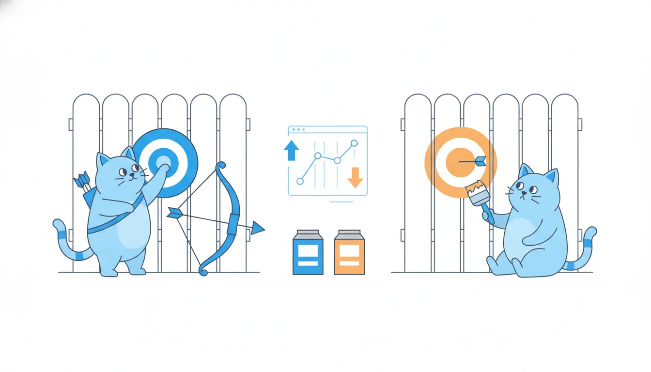
Steps 2 and 3 depend on the data's shape, so looking at histograms before choosing the test is fine. What must come first is the question and the metric, not the answer you hope for.