Pitfalls: peeking, multiple testing, novelty effect

A standard significance test promises a 5% false-positive rate under one condition: you look once, at the sample size you planned.

While a test runs, the p-value wanders. Even when the variant does nothing, it drifts up and down as users arrive, and now and then it dips below 0.05 for a while before recovering. If you check repeatedly and stop the first time it crosses, you're no longer running one test. You're running several and keeping the luckiest.

Simulations of a test with no real effect show how fast this grows. Checking at evenly spaced points and stopping at the first p < 0.05:

• 1 look: about 5%;
• 5 looks: about 14%;
• 10 looks: about 19%;
• 20 looks: about 25%.

Checking a dashboard every few hours easily means dozens of looks.

The fix isn't to stop looking at dashboards; it's to stop deciding from them. Fix the sample size before launch, and treat interim numbers as monitoring, not verdicts, unless you use a method built for repeated looks.

Each test at α = 0.05 has a 5% chance of a false positive. Run several and the chance that at least one fires by accident grows fast. For m independent metrics that truly didn't change:

P(at least one false positive) = 1 − (1 − α)^m

With 5 metrics: 1 − 0.95⁵ = 1 − 0.7738 ≈ 22.6%. With 20 metrics: 1 − 0.95²⁰ ≈ 64.2%. A test report with twenty metrics is more likely than not to contain a "significant" result that means nothing.

This is the multiple comparisons problem. It shows up whenever you slice one test many ways: many metrics, many segments (mobile, desktop, new users, cities), or many variants against one control.

A quick shortcut is m × α (5 × 5% = 25%), and for small numbers it's close. For many metrics it breaks down: 20 × 5% = 100%, which is impossible. Use the formula.

Real metrics are often correlated, so the exact figure differs, but the direction never does: the more you look, the more likely a fluke.

The simplest fix for multiple comparisons is the Bonferroni correction: divide the overall (family-wise) significance level by the number of comparisons m, and hold each test to that stricter bar.

α per test = α family / m

For 5 metrics at a family-wise 0.05: 0.05 / 5 = 0.01. A metric now counts as significant only if its own p-value is below 0.01.

What you gain: the chance of any false positive across the family stays at or below 5%. What you pay: each test needs a stronger signal, so power drops, and with many metrics the bar gets very high (0.05 / 20 = 0.0025).

That cost is why good test plans try to keep m small in the first place:

• name one primary metric before launch and make the decision on it;
• treat the rest as guardrails or exploration, labelled as such;
• for large exploratory sets, softer methods that control the false discovery rate (FDR) keep more power.

Bonferroni is conservative on purpose: better to miss a marginal effect than to celebrate a fluke.

It's worth checking that the Bonferroni correction actually does its job. Use the formula for the chance of at least one false positive, with the corrected threshold:

P(at least one false positive) = 1 − (1 − α per test)^m

For 5 independent metrics at 0.01 each: 1 − 0.99⁵ = 1 − 0.9510 ≈ 4.9%. Without the correction it was 1 − 0.95⁵ ≈ 22.6%. The family-wise risk is back under the 5% you meant to accept.

The result is always a little below the target, because Bonferroni is slightly conservative. For 20 metrics at 0.0025 each: 1 − 0.9975²⁰ ≈ 4.9% again.

The common mistake is to think each metric "still has its 5%" after the correction, or to apply the correction to one metric and forget the others. The protection only works if every metric in the family is held to the same stricter bar.

And remember the trade-off: the overall false-alarm risk dropped from 22.6% to 4.9%, but each metric now needs a clearer signal to be called significant.

Once you've decided to correct for multiple comparisons, every p-value has to be read against the corrected bar, not the familiar 0.05.

There are two equivalent ways to do it:

• compare with α / m: with 10 metrics, the bar is 0.05 / 10 = 0.005. A p-value of 0.008 doesn't clear it; 0.003 does;
• adjust the p-value: multiply it by m (capped at 1) and compare with 0.05. 0.008 × 10 = 0.08, not significant; 0.003 × 10 = 0.03, significant.

Both give the same answer. The adjusted version is handy in reports, because readers can keep using 0.05 as the line.

The trap is reflex: a p of 0.008 looks impressive, far below 0.05, and it's tempting to celebrate. But that metric was one of ten tries, and the correction exists precisely to stop you from celebrating the best of ten.

In a write-up, say which correction you used and how many comparisons it covered: "Bonferroni across 10 metrics, adjusted p = 0.08". That makes the decision checkable.

A novelty effect happens when regular users react to a change simply because it's new: a bright banner gets clicked out of curiosity, a redesigned page gets explored. The reaction is real, but it fades once the change is familiar.

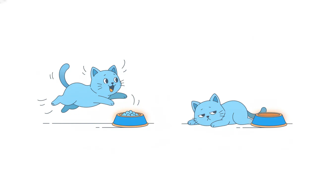
It matters because a test only measures the weeks it runs. If most of the lift sits in week one, the test-period average overstates what you'll see next quarter.

Three checks help:

• plot the effect by week, not just the total. A lift that shrinks steadily (+3, +1, +0.2 points) is the classic shape;
• split new and returning users. New users have no old version to compare with, so a lift that exists only among returning users is a warning sign;
• run full weeks, and long enough for the curve to settle, often at least two to three weeks for a visible change.

The opposite also happens: regular users dislike a change at first, the effect starts negative and recovers. Either way, the stable level later in the test is the better guide to the future than day one or the overall average.

Sometimes there are good reasons to look before the planned end: a broken variant, a big loss, a deadline. There are two honest ways to do it.

Look, but don't decide. Monitor for bugs and disasters (zero conversions, errors, a crash in revenue) and stop for those. Don't stop because the result looks good. The significance decision waits for the planned sample size.

Use a method built for repeated looks. Sequential testing plans the interim checks in advance and spends the 5% error budget across them. A typical schedule demands very strong evidence at early looks (a p-value far below 0.05) and keeps something close to 0.05 for the final one. The overall false-positive rate then stays at 5% however many of the planned looks you take.

What doesn't work is improvising: "two significant days in a row", "stop when the curve flattens", or "one peek is fine". Each of these is a one-look test with extra looks bolted on, and nobody knows its real error rate.

These pitfalls sound alike, but each one asks a different question about a test:

• Peeking (optional stopping): when did you decide? Checking repeatedly and stopping at the first significant moment inflates false positives over time.
• Multiple comparisons: how many things did you test? Many metrics or segments make it likely that one looks significant by chance.
• Novelty effect: would it last? Users react to change itself; the effect is real at first but fades.
• Sample ratio mismatch (SRM): did the split work? If a test planned 50/50 ends with 10,000 users in one group and 10,600 in the other, that gap is far too large for chance (a chi-square test against the expected 10,300 each gives p < 0.001). Something in the assignment or logging is broken, and no result from the test can be trusted until it's found.

In a test review, run through all four in order: split, timing, number of comparisons, durability. A result that survives all four is worth believing.

Most false "winners" come from the process, not the maths. The z-test can be computed perfectly and still mislead if the way you used it gave chance extra tries.

Three classic routes:

• stopping at a lucky moment: peeking daily and ending the test as soon as p dips below 0.05;
• choosing the lucky metric: testing 20 metrics and reporting the one that came out significant. With 20 independent tries, a fluke is more likely than not;
• measuring the excitement: a novelty effect that makes week one look great and then fades.

The protection is boring and effective. Before launch, write down the primary metric, the sample size and the test duration (in full weeks). Run to that sample size. Report every metric you checked, not just the one that worked. Then look at the trend over time before calling the effect permanent.

Notice that "running to the full pre-registered sample size" isn't a pitfall at all: it's the habit that prevents the first one.