Why we square: variance, sums of squares and n − 1

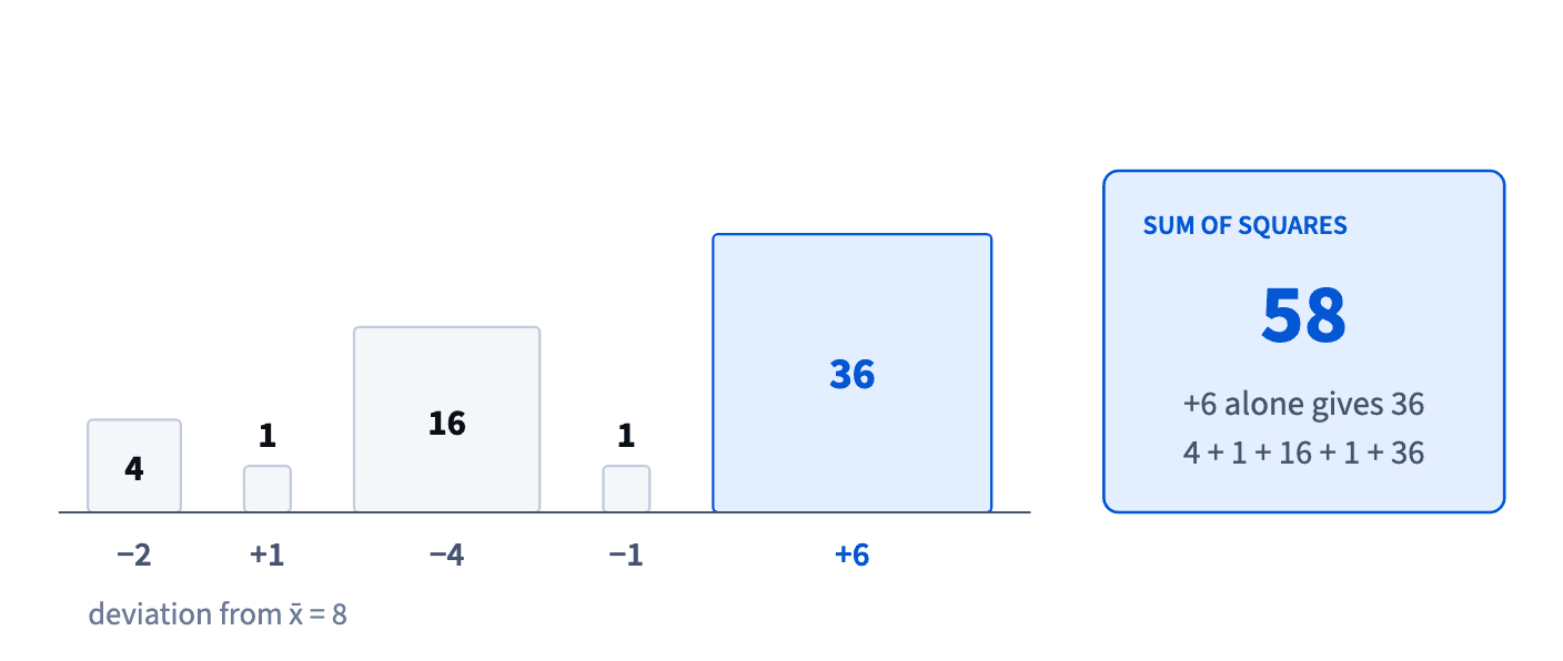
To measure spread, a formula starts from each value's deviation from the mean, x − x̄. Averaging the deviations is useless: deviations from the mean always add up to zero, the Σ rule from The Σ sign: sums, limits and running totals. Five learners with 6, 9, 4, 7 and 14 lessons (mean 8) have deviations −2, +1, −4, −1 and +6, and their sum is 0 however wide the spread.

There are two ways out. Dropping the signs gives the mean absolute deviation: (2 + 1 + 4 + 1 + 6) ÷ 5 = 2.8. Squaring gives 4, 1, 16, 1 and 36, never negative. Statistics mostly squares, for two reasons:

• squares weigh big deviations more, so one far value gets noticed;
• sums of squares split neatly into parts, and tests such as ANOVA rely on that.

The price is the unit. Lessons become "lessons squared", which no one can picture; that's why a square root follows later.

The sum of squares is Σ(xᵢ − x̄)²: square every deviation from the mean, then add. It is the raw material of every spread formula in statistics.

For the five learners with 6, 9, 4, 7 and 14 lessons (mean 8): 4 + 1 + 16 + 1 + 36 = 58. Look at where the 58 comes from. The learner with 14 lessons, 6 above the mean, adds 36 alone, more than the other four together (22).

That's the square at work. A deviation twice as big adds four times as much; three times as big, nine times. Picture each deviation as the side of a square tile: the sum of squares is the total area of the tiles, and one long side makes one huge tile.

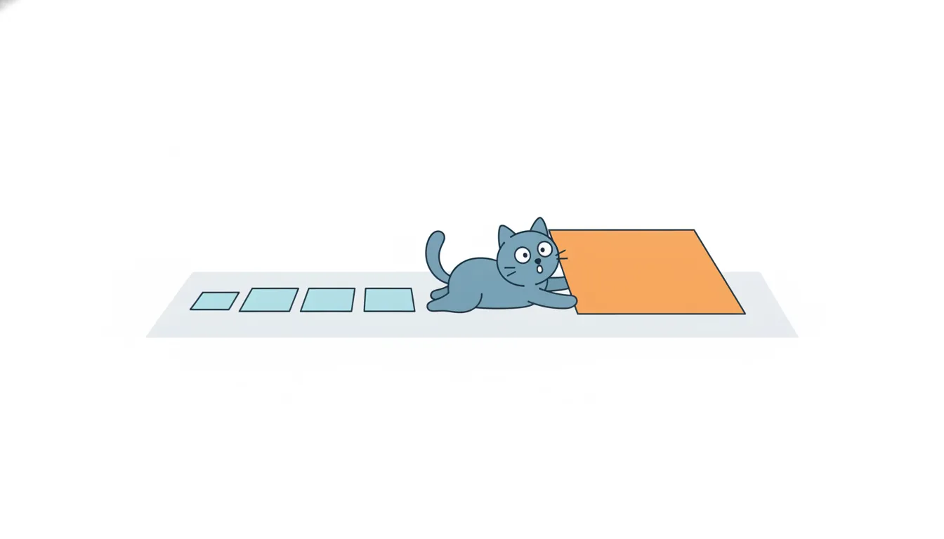
So the sum of squares is sensitive to far values. That helps when a far value matters (one tutor whose learners stop coming) and hurts when it's a data error: a single typo such as 140 instead of 14 would swamp the whole sum. Check the extremes before you trust a variance.

Variance is the sum of squares divided by a count. Which count depends on what your data are.

• s², the sample variance: Σ(xᵢ − x̄)² ÷ (n − 1). Use it when the data are a sample and the question is about a larger group: five learners standing in for all of them, a survey, an A/B test.
• σ², the population variance: Σ(xᵢ − μ)² ÷ N, around the true mean μ. Use it only when you hold every member of the group you ask about, for example the lessons of all 1,120 learners active in March, when the question is about exactly those learners.

Greek letters mark the population and Latin ones the sample, as in Notation: indices, bars, hats and Greek letters. In product work data are almost always a sample, so s² is the default. Spreadsheets carry both: VAR.S divides by n − 1, VAR.P by N.

For the five learners, s² = 58 ÷ 4 = 14.5. Its unit is "lessons squared", which nobody can picture; the next lesson's square root fixes that.

Why does the sample variance divide by n − 1 and not by n? There are two ways to see it.

Free pieces. Deviations from the sample mean must add up to zero. Once you know four of the five learners' deviations, −2, +1, −4 and −1, the fifth is forced: it has to be +6. Only four pieces carry free information. That count, n − 1, is called the degrees of freedom.

A mean fitted to the data. x̄ is computed from the same values, so it sits in their middle by construction, and the data lie a little closer to x̄ than to the true mean μ. The sum of squares around x̄ comes out slightly too small; dividing by n − 1 instead of n makes up for it.

The correction matters most in small samples. With 5 values, ÷ 4 instead of ÷ 5 raises the variance by 25%; with 1,000 values, by 0.1%. It's never a typo, and it isn't a special rule "for small samples": the formula is the same at every size.

Computing s² by hand takes five steps, and doing them in this order prevents most mistakes:

1. Find the mean: x̄ = Σx ÷ n.
2. Subtract it from each value to get the deviations.
3. Check that the deviations add up to 0. If they don't, the mean is wrong.
4. Square each deviation and add: that's the sum of squares.
5. Divide by n − 1.

Example: one Klasna tutor booked 2, 4, 4 and 6 trial lessons in four weeks. x̄ = 16 ÷ 4 = 4. Deviations −2, 0, 0, +2 (sum 0). Squares 4, 0, 0, 4; sum of squares 8. s² = 8 ÷ 3 = 2.67 trial lessons squared.

Typical slips: dividing by n (8 ÷ 4 = 2, the population formula), squaring the values instead of the deviations (4 + 16 + 16 + 36 = 72), and rounding the mean before subtracting it. In a spreadsheet all five steps are one VAR.S; doing them once by hand shows what that function actually does.

Degrees of freedom appear in many formulas, and all of them follow one rule: the number of data pieces minus the number of things estimated from them. Every estimated mean ties one piece down.

• One sample, one mean: n − 1.
• Two samples, two means (the pooled two-sample t-test): n₁ + n₂ − 2.
• Comparing k group means: k − 1 between the groups.
• A table with r rows and c columns: (r − 1)(c − 1), because the row and column totals fix the last cell of every row and column.

They are always counts worked out from sizes, never from the values themselves. Two groups of 10 and 14 learners give 10 + 14 − 2 = 22 degrees of freedom whatever their scores were. A survey table of 4 age groups by 3 answers gives (4 − 1)(3 − 1) = 6.

Why care about the count? Tests later in statistics look up their critical values in a table row chosen by degrees of freedom, so a wrong count means reading the wrong row.

Sums of squares have a property that plain spreads lack: they split exactly into parts.

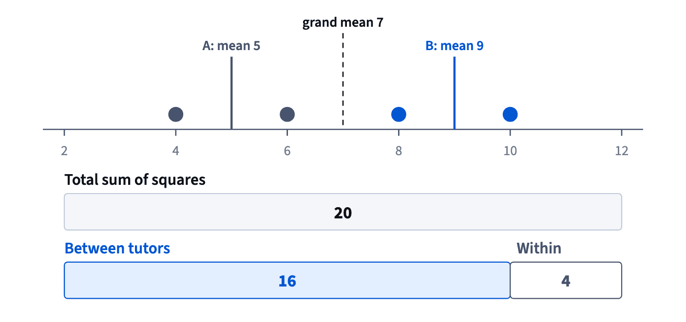
Take two tutors' ratings. A got 4 and 6 (mean 5), B got 8 and 10 (mean 9); the grand mean is 7.

• Total: every value around the grand mean: 9 + 1 + 1 + 9 = 20.
• Between groups: replace each value by its group mean and measure around the grand mean: 2 × (5 − 7)² + 2 × (9 − 7)² = 16. A group mean counts once per member, hence the nⱼ in SS_between = Σ nⱼ(x̄ⱼ − x̄)².
• Within groups: every value around its own group mean: 1 + 1 + 1 + 1 = 4.

And 16 + 4 = 20 exactly. Here most of the spread lies between the tutors, not inside each tutor's ratings. ANOVA is built on this comparison: when the between part is large next to the within part, the groups really differ.

The usual slip is dropping nⱼ: (5 − 7)² + (9 − 7)² = 8, as if each group had one member.

Squares turn up beyond variance. In factor analysis, survey questions are grouped under a few underlying factors, and each question has a loading on a factor: a number from −1 to 1 saying how closely the question follows it. A factor's strength, written λ, is the sum of its squared loadings: λ = Σa².

With loadings 0.8, 0.7 and 0.6: 0.64 + 0.49 + 0.36 = 1.49. Square first, then add. Adding first and squaring the total (2.1² = 4.41) gives a different, wrong number. Squaring also makes the sign irrelevant: a loading of −0.8 adds the same 0.64 as +0.8.

How it fits together: deviations cancel, so we square them; the sum of squares, divided by n − 1 degrees of freedom, becomes the variance, and it splits into between and within parts. The next lesson takes the square root to get back to real units and shows why more data narrows an estimate.