

Theory
Two-sample t-test
The two-sample t-test (Student's t-test): comparing the means of two groups and deciding whether the gap is bigger than chance.
~12 min read · 11 exercises · 250 points
Before you start
Does the upsell widget pay?
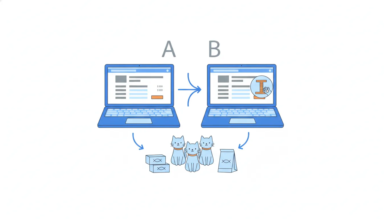
A new question has landed on CatChow's product team. Last week the checkout team showed an upsell widget, offering a scratching post, to half of new sessions. Orders with the widget look bigger on average, and the team is ready to switch it on for everyone. But each group holds only ten orders.
In this lesson you'll learn the two-sample t-test: how to tell whether the gap between two averages is bigger than the noise of sampling.
When the two-sample t-test fits
The two-sample t-test (Student's t-test for independent samples) answers one question: is the gap between the means of two groups bigger than sampling noise would plausibly produce?
It fits when three things are true:
- there are exactly two groups;
- the metric is numeric, and you compare its means: order value, session length, items per basket;
- the groups are independent: different customers, nothing links a particular order in one group to a particular order in the other. A classic A/B test with random assignment gives you exactly that.
Change any of these and you need a different tool:
- the same people measured twice (before and after a price change) are paired samples, which need a test on the per-person differences;
- three or more groups call for ANOVA rather than a pile of pairwise t-tests;
- yes/no outcomes such as churn or conversion are proportions, compared with a z-test for two proportions.
Picking the test is the first decision, and it comes from the design of the experiment, not from the numbers.
- DoUpsell widget shown to a random half of sessions; compare mean order value: two-sample t-test.
Two independent groups, one numeric metric.
- Don'tSame 50 customers before and after a price change → two-sample t-test.
Ignores the pairing, so the test is looser than it should be.
The standard error of a difference
A t-test compares the gap between two means with how much that gap would wobble from sample to sample. That wobble is the standard error of the difference. When both groups have similar spread, the classic test pools their variances first. Take CatChow's upsell widget test: 10 orders per group, with SDs of $3.03 (control) and $3.37 (variant).
- Square each SD to get the variances: 3.03² ≈ 9.18 and 3.37² ≈ 11.36.
- Pool them, weighting by degrees of freedom: sp² = (9 × 9.18 + 9 × 11.36) / 18 ≈ 10.28. With equal group sizes this is simply the average of the two variances.
- Scale by both sample sizes: SE = √(sp² × (1/n₁ + 1/n₂)) = √(10.28 × 0.2) ≈ $1.43.
The SE of a difference is bigger than the SE of either mean alone, because both means wobble and their wobbles add up. Each group here has an SE of about $1, but the difference has $1.43.
Two things shrink it: larger samples (the 1/n terms get smaller) and less noisy metrics (smaller variances). That's why a bigger test or a steadier metric makes small effects easier to detect.
- Dosp² = (9 × 3.03² + 9 × 3.37²) / 18 ≈ 10.28; SE = √(10.28 × 0.2) ≈ 1.43
Variances, not SDs, go into the pooling.
- Don'tPool the SDs: (3.03 + 3.37) / 2 = 3.20, then √(3.20 × 0.2) ≈ 0.80
Skips squaring, so the SE comes out far too small.
The t-statistic: signal over noise
The t-statistic is one division:
t = (x̄₂ − x̄₁) / SE of the difference
The top is the signal: how far apart the two sample means are. The bottom is the noise: how much that gap would wobble if you repeated the experiment with fresh samples. So t says how many standard errors the observed gap is.
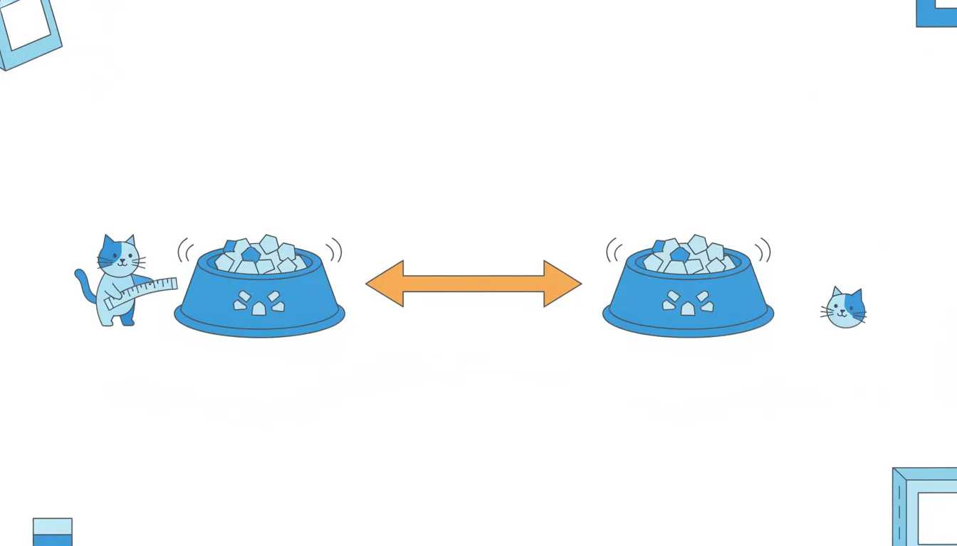
For CatChow's upsell widget test, with means of $52.50 and $42.50: (52.50 − 42.50) / 1.4337 = 10 / 1.4337 ≈ 6.97. The gap is almost seven times larger than its typical wobble.
A few reading tips:
- t near 0 means the gap is small compared with the noise;
- the sign only shows direction. If you subtract the other way round you get −6.97, and the conclusion is the same;
- t has no units. Dollars cancel out, so a t of 2 means the same whether you measured dollars or minutes.
Use the unrounded SE when you can. Rounding the SE to 1.4 first gives 7.14 instead of 6.97: here it doesn't change the verdict, but near a threshold it can.
- Dot = (52.50 − 42.50) / 1.4337 ≈ 6.97
Difference in means over the SE of the difference.
- Don'tt = 10 / 3.20 ≈ 3.13 (dividing by a typical SD)
The SD describes single orders, not how much a mean wobbles.
Degrees of freedom, critical value, verdict
A t-value on its own doesn't tell you whether to reject H0. You compare it with a critical value, which depends on two things.
- The significance level (α): how big a risk of a false alarm you accept. The usual choice is 5%, set before you look at the data.
- The degrees of freedom (df): for the pooled two-sample test, df = n₁ + n₂ − 2. Each group's mean uses up one. With 10 orders per group, df = 18.
A t-table or any statistics software then gives the critical value. For a two-tailed test at 5% with df = 18 it is about 2.101. With more data it shrinks towards 1.96.
The decision rule: if |t| is greater than the critical value, reject H0 (the means are equal) in favour of H1 (they differ). CatChow's upsell widget test (10 orders per group) has |t| = 6.97 > 2.101, so the result is statistically significant.
"Two-tailed" means you would care about a difference in either direction, which is the safe default for product tests.
- Dodf = 10 + 10 − 2 = 18 → critical ≈ 2.101; |6.97| > 2.101 → reject H0.
Compare the absolute t with the critical value for the right df.
- Don'tChoosing α = 10% after seeing t = 1.8, so that the result “counts”.
The threshold must be fixed before the data.
What a significant t lets you say
A significant t-test supports one specific claim: the population means very likely differ. The gap you saw is too large to be explained by sampling noise alone, at the significance level you chose.
It does not tell you:
- the exact size of the effect. The observed $10 is a sample estimate. Another week could show $7 or $13. Later in the course you'll put a confidence interval around it;
- that the effect will last. A novelty effect can fade after launch;
- that the effect matters. Statistical significance is about noise, not money. With a huge sample, even a few cents can be significant;
- why it happened. The test compares outcomes; the cause comes from the experiment design.
A good summary separates these: the verdict ("significant at 5%"), the estimate ("about +$10 per order in this sample"), and the uncertainty ("based on 10 orders per group"). Writing "exactly $10" turns an estimate into a promise, and the next test may break it.
- Do“Significant at 5% (t ≈ 6.97). In this sample, about +$10 per order; 10 orders per group.”
Verdict, estimate and uncertainty kept apart.
- Don't“The widget adds $10 to every order. Forecast: +$10 × all orders next year.”
Treats a small-sample estimate as a fixed, lasting effect.
Hypotheses and the two kinds of error
Every test starts with two competing statements about the populations.
- The null hypothesis (H0): there's no real difference; the two population means are equal and any gap in the samples is noise.
- The alternative hypothesis (H1): the population means differ.
The test never proves H1. It asks whether the data are surprising enough under H0 to reject it. The critical value is the line: a t beyond it is surprising enough, given the significance level and the degrees of freedom.
Because you decide from samples, two mistakes are possible:
- a type I error (false positive): rejecting H0 when there's no real difference. You ship a widget that does nothing. Its probability is capped by α, usually 5%;
- a type II error (false negative): failing to reject H0 when a real difference exists. You kill a feature that works, typically because the sample was too small.
You can't drive both to zero at once with a fixed sample. More data is the main way to reduce type II errors without raising type I.
- Do“H0: mean order value is the same with and without the widget.”
H0 is the boring, no-difference statement.
- Don't“We failed to reject H0, so we proved the widget has no effect.”
Not rejecting H0 may just be a type II error.
A full t-test in five steps
Every pooled two-sample t-test runs the same five steps.
- Pool the variances: sp² = ((n₁ − 1)s₁² + (n₂ − 1)s₂²) / (n₁ + n₂ − 2). With equal SDs of 4, sp² = 16.
- Standard error of the difference: SE = √(sp² × (1/n₁ + 1/n₂)) = √(16 × 0.25) = 2.
- t-statistic: (35 − 30) / 2 = 2.5.
- Degrees of freedom and critical value: df = 8 + 8 − 2 = 14; for a two-tailed test at 5%, about 2.145.
- Verdict: 2.5 > 2.145, so reject H0. The difference is significant at 5%.
Notice how close the call is. With 8 sessions per group, a 5-item gap barely clears the bar; with 4 sessions per group the SE would be 2.83, t ≈ 1.77, and the same gap would not be significant.
The classic slip is in step 2: using the SE of one group (4 / √8 ≈ 1.41) instead of the SE of the difference. That makes t ≈ 3.54 and overstates the evidence, because it ignores that the other mean wobbles too.
- DoSE = √(16 × (1/8 + 1/8)) = 2 → t = 5 / 2 = 2.5
Both groups' uncertainty is in the SE.
- Don'tSE = 4 / √8 ≈ 1.41 → t ≈ 3.54
One group's SE: the evidence looks stronger than it is.
The assumptions behind the classic t-test
The pooled Student's t-test gives trustworthy answers when three assumptions hold.
- Independence. The two samples don't influence each other, and observations within each group are separate. Random assignment in an A/B test usually takes care of this; the same customer counted in both groups breaks it.
- Roughly normal data, or large enough samples. The test is built on means, and the central limit theorem makes means behave normally as samples grow. With 10 orders per group the data itself should look roughly bell-shaped.
- Roughly equal variances. The pooled formula blends the two variances into one. If one group is far noisier than the other, use Welch's version instead.
Formula: Pooled standard error: sp² blends both groups' variances, weighted by their degrees of freedom. · shown above
What's not required: equal group sizes. Uneven splits are fine; the formula adjusts.
The practical danger is outliers. One huge order inflates a mean and its variance, and can create or hide a "significant" difference by itself. Look at the data before trusting a t; if a few extremes drive it, a rank-based test is the safer tool.
- DoGroups of 40 and 55 customers, similar spread, no extreme orders: the pooled t-test is fine.
Unequal sizes don't break anything.
- Don'tRunning a t-test on 10 orders per group where one order is $900.
One outlier can decide the result.
Welch's t-test for unequal variances
The classic Student's t-test pools the two variances into one, which is only fair if they're similar. When one group is much noisier, pooling misstates the standard error. It's worst when the smaller group has the bigger variance: the pooled SE comes out too small, and the test produces more false alarms than α promises.
Welch's t-test fixes this. It keeps each group's variance separate:
SE = √(s₁² / n₁ + s₂² / n₂)
and uses an adjusted, usually non-integer, number of degrees of freedom, which software computes for you. Everything else, the t-statistic and the decision rule, works the same way.
When should you use it? Whenever the spreads clearly differ, as with $8 vs $25. Many analysts simply use Welch by default: when the variances happen to be equal, it gives almost the same answer as the pooled test, so you lose very little and gain protection.
Welch doesn't fix outliers or heavy skew, though. If a few extreme values drive the means, switch to a rank-based test.
- Dos = $8 (n = 40) vs s = $25 (n = 15) → Welch: SE = √(64/40 + 625/15) ≈ $6.58.
Each group keeps its own variance.
- Don'tPooling anyway: sp² ≈ 212, SE ≈ $4.41.
The noisy small group gets diluted, so the SE is too small.
Ready to practise?
Answer the lesson's exercises and earn 250 points the first time you finish it.
Start the exercises