

Theory
Measures of spread: range, SD and quartiles
Two couriers with the same average delivery time, and why only one keeps the promise: measures of spread from range and variance to standard deviation (calculated step by step), quartiles, IQR and the coefficient of variation.
~11 min read · 11 exercises · 250 points
Before you start
Two couriers, one average
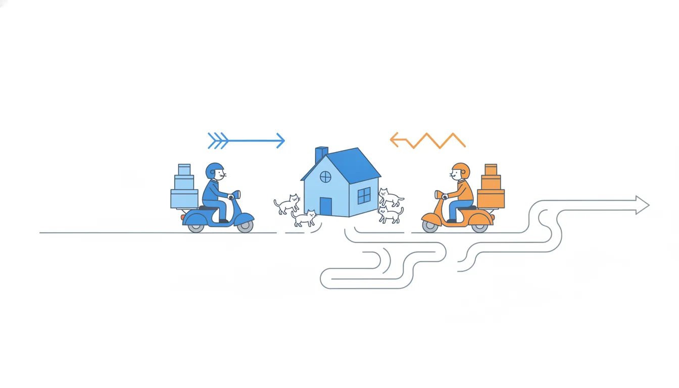
You're still on CatChow's product team. Today the question comes from operations: the shop works with two courier companies, customers are promised delivery within 36 hours, and the operations lead wants to drop one of them. Her argument is that both average exactly 24 hours, so it doesn't matter which one stays.
In this lesson you'll check that claim against the delivery data and learn to measure how far single values stray from the average: range, standard deviation and quartiles.
Standard deviation, step by step
The standard deviation (SD) measures how far a typical value sits from the mean, in the units of the data. It takes six steps:
- Find the mean.
- Subtract it from each value to get the deviations.
- Square each deviation, so negatives stop cancelling positives.
- Add up the squares.
- Divide by n − 1 to get the sample variance.
- Take the square root.
Courier A's 10 deliveries average 24 hours. The deviations are −3, −3, −1, −1, 0, 0, +2, +2, +2, +2; the squares add up to 36; 36 / 9 = 4; √4 = 2 hours. Courier B, with the same mean, gets 576 / 9 = 64 and an SD of 8 hours.
Chart data
| Delivery time, hours | Courier A | Courier B |
|---|---|---|
| 12–15 | 0 | 2 |
| 16–19 | 0 | 2 |
| 20–23 | 4 | 0 |
| 24–27 | 6 | 2 |
| 28–31 | 0 | 3 |
Show 2 more rows
| 32–35 | 0 | 0 |
| 36–39 | 0 | 1 |
Dataset · 20 rows
CatChow deliveries by courier
The last 10 deliveries by each of two couriers. Synthetic data made for this course.
First 5 of 20 rows
Why n − 1? Ten deliveries are a sample, and the sample mean sits a little closer to its own values than the true long-run mean does. Dividing by 9 instead of 10 corrects for that. In a spreadsheet, STDEV.S is the sample version and STDEV.P the population one.
- DoCourier A: 36 / 9 = 4, √4 = 2 hours.
Sum of squares, divide by n − 1, then the root.
- Don'tCourier A: 36 / 9 = 4, so the SD is 4 hours.
Stops at the variance and forgets the square root.
Quartiles and the interquartile range
The median splits sorted data in half; quartiles split it into quarters. Q1 has a quarter of the values below it, Q2 is the median, Q3 has three quarters below it.
A simple way to find them by hand:
- Sort the values.
- Split them into a lower and an upper half.
- Q1 is the median of the lower half, Q3 the median of the upper half.
Courier A, sorted: 21, 21, 23, 23, 24 | 24, 26, 26, 26, 26. The lower half's median is 23, the upper half's is 26.
Dataset: CatChow deliveries by courier · shown above
The interquartile range (IQR) is Q3 − Q1 = 26 − 23 = 3 hours: the width of the middle 50% of deliveries. Courier B's IQR is 30 − 18 = 12 hours.
The IQR ignores the extremes completely, which makes it the natural spread partner of the median. Spreadsheet QUARTILE functions interpolate and can give slightly different quartiles on other data; that's fine, as long as you use one method when comparing groups.
- DoQ1 = median(21, 21, 23, 23, 24) = 23; Q3 = median(24, 26, 26, 26, 26) = 26; IQR = 3.
Medians of the two halves, then the difference.
- Don'tIQR = 26 − 21 = 5
That's the range: largest minus smallest.
Variance and its squared units
To measure spread from every value, you start with deviations: each value minus the mean. Their plain average is useless, because the mean is the balance point of the data and the deviations always add up to zero.
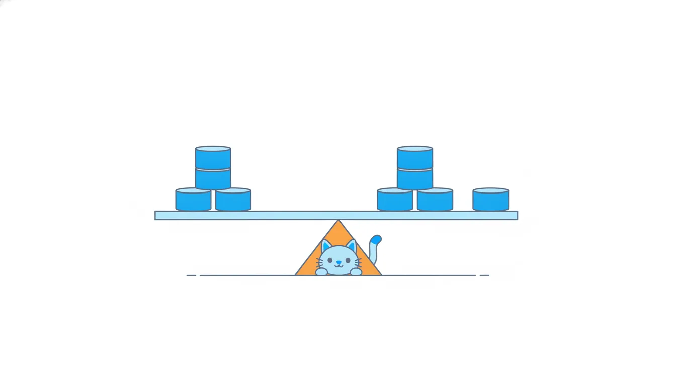
The fix is to square them. Squares are never negative, and big misses count far more than small ones: a deviation of 14 becomes 196. The average of the squared deviations (dividing by n − 1 for a sample) is the variance. For courier B's 10 deliveries (mean 24 hours) it's 576 / 9 = 64.
Squaring has a side effect: the units are squared too. Courier B's variance is 64 hours², a unit nobody can picture. Order values would give a variance in "dollars squared".
That's why reports use the standard deviation, the square root of the variance: √64 = 8 hours, back in normal units. The two carry the same information. Variance is the convenient form inside formulas and tests; the SD is the one you put in front of people, written next to the mean: "24 ± 8 hours".
- Do“Variance 64 hours², SD 8 hours: deliveries are typically about 8 hours from the mean.”
Squared units for the variance, normal units for the SD.
- Don't“Deliveries vary by about 64 hours.”
Reads the variance as if it were in hours.
Why the steps go in this order
Each step of the standard deviation fixes a problem left by the step before it.
- Mean: you need a centre to measure distances from.
- Deviations: value minus mean, one distance per value. Their sum is always zero, so you can't stop here.
- Squares: they remove the signs and make large misses count more.
- Sum: one number for the whole dataset.
- Divide by n − 1: turns the sum into an average squared distance, the sample variance. The n − 1 corrects for the sample mean sitting a bit too close to its own data. With the whole population, divide by n.
- Square root: undoes the squaring of the units, giving the SD in hours, dollars or minutes.
Swapping steps breaks the result. Taking the root before dividing, or averaging the deviations before squaring them, gives a different number that has no meaning. A quick sanity check: the SD can't be negative, and for most data it is smaller than the range divided by 2.
- DoMean → deviations → squares → sum → ÷ (n − 1) → √
- Don'tAverage the deviations first: (−10 − 10 − 6 − 6 + 0 + 0 + 6 + 6 + 6 + 14) / 10 = 0
Deviations always cancel out, so this says “no spread” every time.
Which spread measures an outlier breaks
Measures of spread differ in how much one extreme value can move them.
- Range uses only the two most extreme values, so one strange value changes it directly.
- Variance and SD use every value, and squaring makes big deviations count even more. One far-off value can dominate the whole sum of squares.
- IQR depends only on the middle half of the sorted data, so the extremes don't enter it at all.
Measures of spread: which one to use when
Back to the couriers. Courier A: range 5 hours, and every delivery within the promise. Courier B: range 24 hours, SD 8 hours, IQR 12 hours, and 1 of 10 deliveries late. Same average, very different customer experience. The case task at the end asks you to make the call.
Add one lost parcel of 90 hours to courier A's 10 deliveries. The range jumps from 5 to 69 hours. The SD jumps from 2 to about 20 hours, and the variance from 4 to about 400. The IQR stays at 3 hours, because Q1 and Q3 barely move.
That's why spread measures come in pairs with centre measures: mean with SD, median with IQR. When the data has a long tail or a few freak values, report the median and IQR (or percentiles) for the typical experience, and look at the extremes separately.
- Do“Courier A: median 24 h, IQR 3 h; one lost parcel at 90 h, investigated separately.”
Robust measures for the typical case, the outlier named.
- Don't“Courier A's SD jumped from 2 to 20 hours, so it became unreliable.”
One parcel did that; the other ten deliveries didn't change.
The coefficient of variation
Is an SD of 8 big? It depends on the scale. Eight hours is a lot for a 24-hour delivery and nothing for a 30-day subscription cycle. And an SD in dollars can't be compared with an SD in sign-ups at all.
The coefficient of variation (CV) fixes both problems: divide the SD by the mean, usually as a percentage.
CV = SD / mean
Daily ad spend with a mean of $2,000 and an SD of $200 has a CV of 10%. Daily sign-ups with a mean of 50 and an SD of 15 have a CV of 30%. Spend is steady, but results swing three times as much relative to their size. That's a hint that something other than budget, such as the day of the week or the creatives, drives sign-ups.
Use CV only for values measured from a true zero: hours, money, counts. For metrics that can be negative or have an arbitrary zero, such as NPS or temperature, the ratio is meaningless.
- DoSpend 200 / 2,000 = 10%; sign-ups 15 / 50 = 30%: sign-ups are three times as variable.
Both SDs scaled by their own means.
- Don't“Spend varies more: its SD is 200, sign-ups only 15.”
Compares dollars with people.
Reading “mean ± SD”
"24 ± 8 hours" is the most common way to report a centre with its spread. It's worth reading it carefully.
The SD is the typical distance from the mean, not a minimum or a maximum. Some values are closer, some are further away. For data that forms a roughly symmetric hill, a rule of thumb helps: about 68% of values fall within one SD of the mean and about 95% within two.

Courier B: one SD around 24 hours is 16 to 32 hours, and 7 of the 10 deliveries fall there. Two SDs is 8 to 40 hours, and all ten do. The 36-hour promise sits inside the two-SD band, so occasional late deliveries are expected, not a fluke.
Two cautions. First, the rule assumes a bell-ish shape; for skewed data, use percentiles instead. Second, ten values are too few to trust the percentages exactly. Still, "24 ± 8 hours" tells a manager far more than "24 hours on average": it says how much a customer's experience can differ from the headline number.
- Do“24 ± 8 hours: most deliveries arrive within about a day and a third; a few take up to 38 hours.”
SD as a typical distance, extremes named.
- Don't“With SD 8, no delivery can take longer than 32 hours.”
Treats one SD as a hard limit.
Sample or population: n − 1 or n
There are two versions of the variance and the SD, and they differ only in step 5.
- Sample (the default in product work): divide the sum of squares by n − 1. Use it when your data is a slice of something bigger: five weeks of a programme that will run for months, 500 orders out of all orders.
- Population: divide by n. Use it only when you have every value you care about and don't want to generalise.
Formula: Left: sample variance (divide by n − 1). Right: population variance (divide by N, deviations from the population mean μ). · shown above
The sample version is a little larger. That's on purpose: the sample mean is computed from the same values, so the deviations from it come out slightly too small, and n − 1 compensates.
With 5 weekly values of 12, 15, 9, 18 and 6, the mean is 12 and the squares add up to 90. Sample: 90 / 4 = 22.5, SD ≈ 4.74. Population: 90 / 5 = 18, SD ≈ 4.24.
The gap shrinks as n grows, but with small samples it is noticeable. When a dashboard shows an SD, check which version it uses.
- Do90 / (5 − 1) = 22.5, √22.5 ≈ 4.74
Five weeks are a sample of the programme's life.
- Don't90 / 5 = 18, √18 ≈ 4.24
Population formula on a sample: understates the spread.
Percentiles: the experience the average hides
A percentile is the value below which a given share of the data falls. The 90th percentile, or p90, is the time within which 90% of deliveries arrive; the remaining 10% take longer. Quartiles are special percentiles: Q1 is p25, the median is p50, Q3 is p75.
Product teams use high percentiles for promises and service levels: "p90 delivery time is 30 hours", "p95 page load is 2.8 seconds". They answer the question averages can't: how bad is it for the customers who wait longest?
Compare the alternatives:
- the mean describes the centre, not the tail;
- the maximum is one value, so a single lost parcel becomes the whole metric;
- the SD mixes fast and slow deviations and swings with one extreme value.
A high percentile sits between them: it focuses on the slow end, yet one freak value among hundreds hardly moves it. With very few values (say 10 deliveries) p90 is shaky, so collect enough data before setting a target on it.
- Do“p90 delivery time: 30 hours; target: under 36.”
Describes the slow end and links it to the promise.
- Don't“Worst delivery this month: 90 hours, so our service is failing.”
One lost parcel is treated as the whole picture.
Ready to practise?
Answer the lesson's exercises and earn 250 points the first time you finish it.
Start the exercises