

Theory
Repeated measures ANOVA
Tracking the same users across several points in time with a repeated measures ANOVA or the Friedman test.
~11 min read · 11 exercises · 250 points
Before you start
Three checkpoints
Same loyalty program, same CatChow product team. Now you're tracking monthly orders for the same five subscribers at three points in time: signup week, week 4 and week 8. A paired test for every pair of checkpoints would bring back the multiple-comparisons problem.
This lesson closes the module with repeated-measures ANOVA, one test for the same people measured several times, and its rank-based alternative.
More than two checkpoints: repeated measures
When the same subjects are measured at three or more points, say monthly orders for 5 loyalty subscribers at signup, week 4 and week 8, you have a repeated-measures (within-subjects) design. It's the before/after idea extended in time.
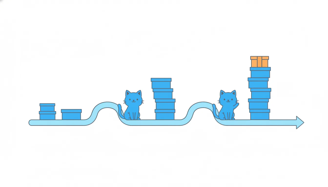
The tempting analysis is a paired t-test for every pair of checkpoints: week 0 vs 4, week 4 vs 8, week 0 vs 8. That's three tests, and the same multiple comparisons problem as running three t-tests instead of a one-way ANOVA: if nothing really changed, the chance that at least one fires anyway is about 1 − 0.95³ ≈ 14%.
Repeated-measures ANOVA answers the broad question in one go: do the means differ across time points at all? It keeps one honest 5% error rate, and it keeps the big advantage of pairing: each subject is compared with themselves.
If the overall test is significant, pairwise follow-ups come next, with a correction such as Bonferroni (0.05 / 3 ≈ 0.0167 for three pairs).
- Do“Three checkpoints, same 5 subscribers: one repeated-measures ANOVA, then corrected pairwise checks if needed.”
- Don't“Three paired tests at 0.05; week 4 vs week 8 came out significant.”
Three uncorrected tries inflate the false-positive rate.
Three slices instead of two
One-way ANOVA splits the variation in the data into two parts: between groups and within groups. Repeated-measures ANOVA splits it into three:
SS_total = SS_subjects + SS_time + SS_error
- subjects: how much subscribers differ from each other overall. U1 averages 6 orders a month, U5 averages 14. That's real, stable, and not what we're testing;
- time: how much the checkpoint means differ (7, 10 and 13 orders). This is the effect of interest;
- error: what's left, the part of each subscriber's movement that doesn't follow the common trend.
Chart data
| Checkpoint | U1 | U2 | U3 | U4 | U5 |
|---|---|---|---|---|---|
| Week 0 | 2 | 6 | 7 | 8 | 12 |
| Week 4 | 6 | 7 | 11 | 13 | 13 |
| Week 8 | 10 | 11 | 12 | 15 | 17 |
The key move is the subjects slice. In a design with different people at each checkpoint, those personal differences would sit in the error term and blur the time effect. Here every subscriber appears at every checkpoint, so their personal level can be measured and removed.

It's exactly what the paired t-test did with differences, generalised: instead of subtracting "before" from "after", the analysis subtracts each subject's own average level.
- Do220 = 120 (subjects) + 90 (time) + 10 (error)
- Don't220 = 90 (time) + 130 (error), ignoring who is who
Leaves the subject differences inside the noise.
Computing the sums of squares
With 5 subscribers at 3 checkpoints, the grand mean is 10 orders a month.
- SS_total: squared deviations of all 15 numbers from 10, added up: 220.
- SS_subjects: each subscriber's mean (6, 8, 10, 12, 14) minus 10, squared, times the 3 checkpoints: 3 × (16 + 4 + 0 + 4 + 16) = 120.
- SS_time: each checkpoint mean (7, 10, 13) minus 10, squared, times the 5 subscribers: 5 × (9 + 0 + 9) = 90.
- SS_error: whatever is left: 220 − 120 − 90 = 10.
Notice the weights: a subject mean summarises 3 numbers, so it's multiplied by 3; a time mean summarises 5, so it's multiplied by 5. Forgetting those multipliers is the usual slip, and it makes the error term come out absurdly large (220 − 40 − 18 = 162).
The small error here says something concrete: once you know who the subscriber is and which checkpoint it is, there's very little left to explain. The subscribers move almost in lockstep.
- DoSS_error = 220 − 120 − 90 = 10
- Don'tSS_error = 220 − 90 = 130
Forgets to take out the subjects slice.
Degrees of freedom and F for repeated measures
Each sum of squares gets its own degrees of freedom, with n subjects and k checkpoints:
- subjects: n − 1 = 5 − 1 = 4;
- time: k − 1 = 3 − 1 = 2;
- error: (n − 1)(k − 1) = 4 × 2 = 8.
The F-statistic for the time effect compares the time mean square with the error mean square:
- MS_time = 90 / 2 = 45;
- MS_error = 10 / 8 = 1.25;
- F = 45 / 1.25 = 36.
The critical F at α = 0.05 for df(2, 8) is about 4.46, so F = 36 is far beyond it (p ≈ 0.0001). Orders clearly change across the checkpoints.
Note that the error has only 8 degrees of freedom, fewer than the 12 an independent-groups analysis of 15 numbers would use. Pulling out the subjects costs 4 degrees of freedom. It's a good trade whenever subjects differ a lot from each other, as they do here: the error mean square shrinks far more than the df do.
The subjects row usually isn't tested at all: nobody doubts that people differ.
- DoF = (90 / 2) / (10 / 8) = 45 / 1.25 = 36
- Don'tF = (90 / 2) / (10 / 12) = 54
Uses the independent-groups df (12) for the error instead of (n − 1)(k − 1) = 8.
Same 15 numbers, two very different F values
Take CatChow's monthly orders for 5 loyalty subscribers at 3 checkpoints: SS_total = 220, SS_subjects = 120, SS_time = 90, so MS_time = 45. Analyse them the naive way, as if each week had different people:
- error SS = SS_total − SS_time = 220 − 90 = 130, on 15 − 3 = 12 df;
- MS_error = 130 / 12 ≈ 10.83;
- F = 45 / 10.83 ≈ 4.15, against a critical value of about 3.89 for df(2, 12). Barely significant, p ≈ 0.04.
Now the repeated-measures way: the subjects' 120 comes out of the error, leaving 10 on 8 df, MS_error = 1.25 and F = 36, p ≈ 0.0001.
The time effect is identical in both (MS_time = 45). Only the noise changed. In the naive version, the fact that U5 always orders more than U1 is counted as random noise, and it dwarfs the trend. In the repeated-measures version it's recognised as a stable trait and set aside.

With slightly noisier data, the naive analysis would have missed the effect altogether. So when the same people are measured repeatedly, the subject term isn't optional: leaving it out throws away the power the design gave you, and it also breaks the independence assumption of the simpler test.
- DoNaive: 45 / (130 / 12) ≈ 4.15. Repeated: 45 / (10 / 8) = 36.
- Don't“F ≈ 4.15 is significant anyway, so the simpler analysis is fine.”
It ignores the pairing and violates independence; it got lucky here.
Repeated measures vocabulary
Four terms you'll meet together:
- repeated-measures ANOVA: ANOVA for three or more measurements on the same subjects, with the between-subject variability removed from the error term;
- Friedman test: its non-parametric alternative. It ranks each subject's own measurements (1st, 2nd, 3rd) and compares the rank sums across time points;
- cohort: a group of users who share a starting event in the same period, for example everyone who joined the loyalty program in the same week. Repeated measures are a natural fit for following one cohort over time;
- degrees of freedom (df): the number of values free to vary once the estimated quantities are fixed. In repeated measures the error gets (n − 1)(k − 1).
One practical warning about cohorts: if some subscribers drop out before week 8, the classic analysis needs every subject at every checkpoint. Dropping incomplete subjects quietly can bias the result toward the people who stayed, often the happiest ones. Report how many subjects were lost and why.
- Do“Cohort: 5 subscribers who joined in week 1, all present at weeks 0, 4 and 8.”
- Don't“Two subscribers left before week 8, so we just analysed the rest.”
Silent drop-outs bias the trend toward the users who stayed.
The Friedman test: ranks within each subject
The Friedman test is the rank-based alternative to repeated-measures ANOVA. Its trick is to rank within each subject, never across subjects, so a heavy buyer and a light buyer count the same.
- For each subscriber, rank their own checkpoints: lowest = 1, highest = 3. U1's 2, 6, 10 become 1, 2, 3. Every subscriber here rises, so every row is 1, 2, 3.
- Add the ranks per checkpoint: R = 5, 10, 15.
- Compute Q = 12 / (n·k·(k + 1)) × ΣR² − 3n(k + 1) = 12 / 60 × 350 − 60 = 10.
- Compare with a chi-square distribution with k − 1 = 2 df: the 5% critical value is about 5.99. Q = 10 is beyond it, p ≈ 0.007.
If time didn't matter, ranks would scatter and each checkpoint's sum would be near n(k + 1) / 2 = 10.
Because only the order within a subject counts, one wild value (an NPS crash from 20 to −20 after a billing error) moves that subject's ranks by at most a step or two instead of dominating the means. The price, as always with ranks, is a little less power on clean data.
- DoQ = 0.2 × (25 + 100 + 225) − 60 = 70 − 60 = 10 > 5.99
- Don'tRank all 15 numbers together from 1 to 15, then compare weeks.
Ranking across subjects brings the subject differences back in.
Why repeated measures needs fewer people
Put the facts of a repeated-measures design side by side:
- the same subjects at every point. That's the definition; different people at each checkpoint would be independent groups;
- fewer error degrees of freedom: (n − 1)(k − 1) = 8 here, against N − k = 12 for independent groups. A small cost;
- a much smaller error term: MS_error = 1.25 instead of about 10.83, because the stable differences between subscribers are removed. A big gain;
- so, more power: the same 15 numbers give F = 36 instead of about 4.15. To reach the same power with independent groups you'd need many more people.
That's why product teams like within-subjects designs for tracking cohorts, comparing a user's behaviour before and after onboarding changes, or testing several versions with the same panel of users.
The main costs are practical rather than statistical: people drop out over time, earlier measurements can influence later ones (learning, fatigue), and without a comparison group a common trend over time, like a season, looks just like an effect.
When the data are skewed or the sample tiny, the Friedman test is the rank-based fallback.
- Do“Same 5 subscribers at 3 points: error df = 4 × 2 = 8, F(2, 8) = 36.”
- Don't“Repeated measures needs a new sample at each checkpoint to stay independent.”
Reusing the same subjects is the design, not a flaw.
Reporting a repeated-measures result honestly
A strong repeated-measures result answers one question well: do the values change over time for the same people? It doesn't answer two others.
How big is the change? F = 36 says the change is far larger than the noise, not that it's large for the business. Report the means and the difference: 7 → 10 → 13 orders a month, about +6 from signup to week 8. Then judge whether +6 orders justifies the program's cost.
What caused it? Every subscriber was in the program the whole time, so time and treatment are tangled together. New customers often order more as they settle in; seasons shift; prices change. Without a comparison cohort that didn't get the program, or a randomised rollout, the honest wording is "orders rose over the period", not "the program raised orders".
A good summary line: the change with its size, the test result, and the main caveat: "+6 orders/month from signup to week 8 (F(2, 8) = 36, p ≈ 0.0001); no comparison group, so part may be the usual new-customer ramp-up."
- Do“+6 orders/month over 8 weeks, F(2, 8) = 36; causation unproven without a comparison cohort.”
- Don't“F = 36, so the program works 36 times better.”
F is a signal-to-noise ratio, not the size of the effect.
Ready to practise?
Answer the lesson's exercises and earn 250 points the first time you finish it.
Start the exercises