

Theory
One-way ANOVA: comparing many groups
Testing three or more variants at once with a one-way ANOVA, without inflating false positives.
~11 min read · 11 exercises · 250 points
Before you start
Three emails, one test
Still at CatChow, on the product team, with a new module and a new test to read. Marketing has tested three welcome emails for new users, the Classic, the Playful and the Discount-first, and everyone expects the discount to win.
Comparing three groups two at a time quietly raises the chance of a false alarm. In this lesson you'll learn one-way ANOVA, a single test for three or more groups at once.
Why not just run a t-test for every pair?
With three email variants there are three pairs: Classic vs Playful, Playful vs Discount-first, Classic vs Discount-first. Running a t-test on each looks thorough, but every test carries its own 5% risk of a false alarm.

If no variant really differs, the chance that at least one of three tests fires anyway is about 1 − 0.95³ ≈ 14.3%, almost three times the 5% you meant to accept. With four variants there are six pairs, and the risk climbs to about 1 − 0.95⁶ ≈ 26.5%. (The pairwise tests share data, so the exact figures differ a little, but the inflation is real.)
This is the multiple comparisons problem again, now inside a single test. The fix is to ask the broad question first, with one test: are all the group means equal? That's what one-way analysis of variance (ANOVA) does, with one F-statistic and one honest 5% error rate.
Only if that overall answer is "no" do you move on to pairs, using a method that keeps the combined error rate in check.
- Do“Three variants, so one one-way ANOVA first; pairs only if it’s significant.”
- Don't“Three t-tests at 0.05; one came out significant, so we have a winner.”
Three tries make a fluke about three times as likely.
What one-way ANOVA tests
One-way analysis of variance (ANOVA) compares the means of three or more groups that differ by one factor, here the email variant.
Like every test, it starts from a null hypothesis:
- H0: all population means are equal (μ Classic = μ Playful = μ Discount-first);
- H1: at least one mean differs from the others.
Note what H1 does not say: it doesn't say all means differ, and it doesn't say which one is different. Rejecting H0 only tells you the "all equal" story doesn't fit the data.
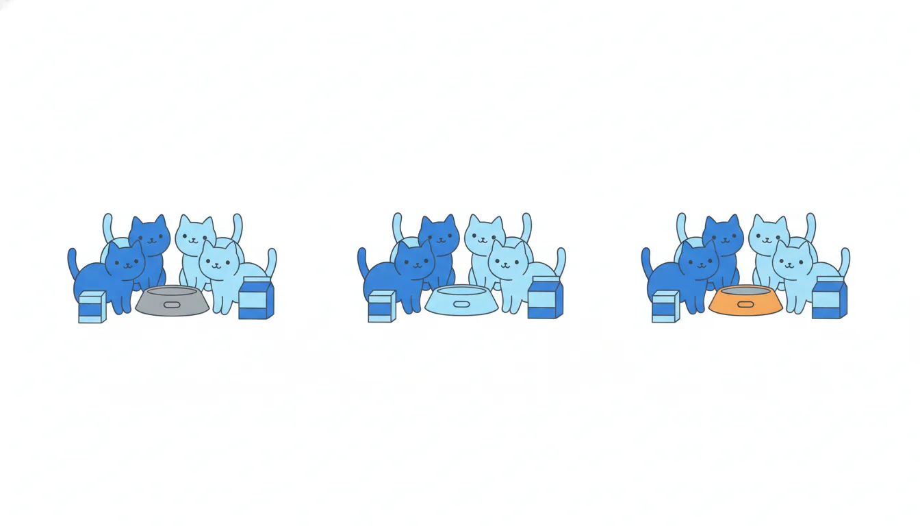
The name sounds odd for a test about means. It comes from how the test works: it compares two kinds of variance. If the variants truly didn't matter, the group means would differ only by about as much as random noise between users allows. If they differ much more than that, H0 becomes hard to believe.
That's why the result of an ANOVA is always a two-step story: first "are the means all equal?", and only then, if not, "which ones differ?"
- DoH0: μ1 = μ2 = μ3. H1: at least one μ differs.
- Don'tH1: μ1 ≠ μ2 ≠ μ3 (“all three are different”).
A significant ANOVA can come from just one group standing out.
Computing F from sums of squares
ANOVA splits the total variation in the data into two parts and compares them:
- between-group variance: how far the group means sit from the grand mean. For CatChow's welcome-email test (three variants, 5 users each, mean first-month spend $20, $25 and $30, grand mean $25), SS_between = 5 × ((20 − 25)² + 0² + (30 − 25)²) = 250;
- within-group variance: how far users sit from their own group's mean, the noise. Here SS_within = 30.
Chart data
| Email variant | Mean spend |
|---|---|
| Classic | 20 |
| Playful | 25 |
| Discount-first | 30 |
Sums of squares grow with the number of terms, so each is divided by its degrees of freedom to get a mean square (MS):
- df_between = k − 1 = 3 − 1 = 2, so MS_between = 250 / 2 = 125;
- df_within = N − k = 15 − 3 = 12, so MS_within = 30 / 12 = 2.5.
The F-statistic is their ratio:
F = MS_between / MS_within = 125 / 2.5 = 50
If the variants made no difference, F would hover around 1. Here the gaps between variants are 50 times bigger than the noise would explain. The usual slip is dividing the sums of squares directly: 250 / 30 ≈ 8.3 ignores the degrees of freedom and understates F six times over.
- DoF = (250 / 2) / (30 / 12) = 125 / 2.5 = 50
- Don'tF = 250 / 30 ≈ 8.3
Divides the sums of squares without their degrees of freedom.
Reading F against its critical value
A second worked example, start to finish. Three checkout layouts, 4 users each, means $40, $44 and $48, SS_within = 54.
- Grand mean (equal groups): (40 + 44 + 48) / 3 = 44.
- SS_between = 4 × ((−4)² + 0² + 4²) = 4 × 32 = 128.
- df_between = 3 − 1 = 2, so MS_between = 64.
- df_within = 12 − 3 = 9, so MS_within = 54 / 9 = 6.
- F = 64 / 6 ≈ 10.67.
Whether that's large depends on the degrees of freedom. The critical F at α = 0.05 is about 4.26 for df(2, 9) and about 3.89 for df(2, 12). Since 10.67 is far above 4.26, the result is significant (p ≈ 0.004).
Note that smaller samples need a bigger F: fewer users per group means a noisier estimate of the within-group variance, so the bar rises.
Two slips to avoid: forgetting to multiply by n in SS_between (32 instead of 128 gives F ≈ 2.67, not significant), and using N − 1 instead of N − k for df_within.
- DoF = (128 / 2) / (54 / 9) = 64 / 6 ≈ 10.67 > 4.26
- Don'tSS_between = 32, F = 16 / 6 ≈ 2.67
Forgets to multiply by the 4 users per group.
From “not all equal” to “which one”
A significant ANOVA is a gate, not a verdict. It rules out "all variants perform the same", and that's all.
Many different patterns produce the same significant F:
- one variant far above two similar ones;
- one variant far below two similar ones;
- three evenly spaced variants, as in the email test.
Each pattern leads to a different decision, so the next step is always a post hoc test that compares the pairs while keeping the overall false-positive rate near 5%. For the email test, Tukey's HSD shows that all three pairs differ: Discount-first beats both others, and Playful beats Classic.
Post hoc test · shown above
Only then can you say "Discount-first is best", and even then, add the size of the gap ($30 against $25 and $20) and whether it's worth the cost of the discount.
Chart: Average first-month spend by variant · shown above
The tempting shortcut is to read the winner straight off the bar chart once F is significant. Sometimes that works; sometimes the top two are statistically tied, and the post hoc step is what tells you which case you're in.
- Do“Significant ANOVA, then Tukey: Discount-first beats both, by $5 and $10 per user.”
- Don't“F is significant and Discount-first has the tallest bar, done.”
The tallest bar may still be tied with the second one.
Bonferroni for pairwise follow-ups
Once ANOVA says the means aren't all equal, you'll want to compare pairs. With k groups there are k(k − 1) / 2 pairs:
- 3 groups: 3 pairs;
- 4 groups: 6 pairs;
- 5 groups: 10 pairs.
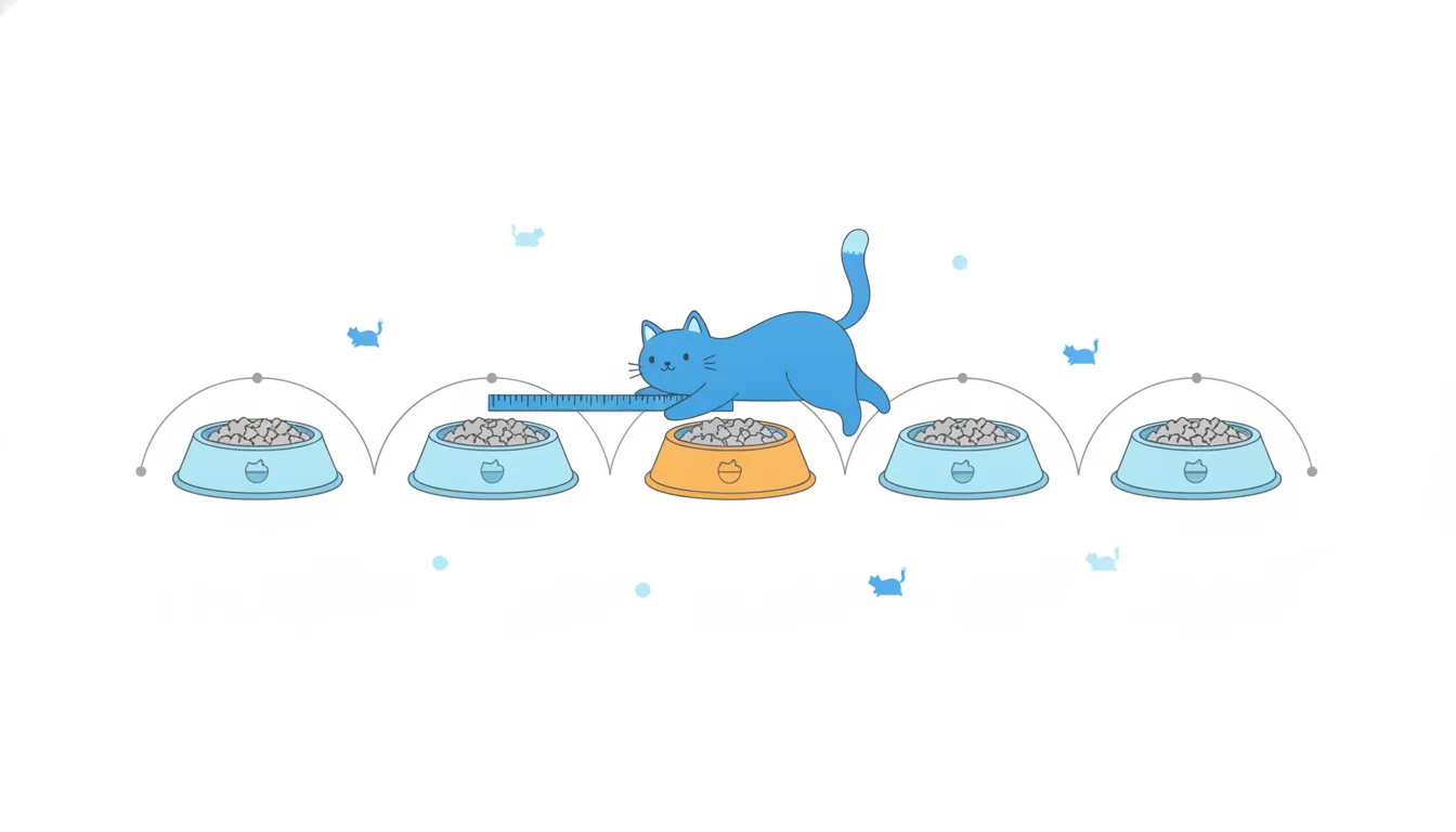
Each pair is another test, so the multiple comparisons problem returns. The simplest guard is the Bonferroni correction: divide the family-wise α by the number of comparisons.
For the three email variants: 0.05 / 3 ≈ 0.0167. A pair counts as different only if its p-value is below 0.0167. With four banner designs it would be 0.05 / 6 ≈ 0.0083.
Bonferroni is easy to apply and easy to explain, which makes it a good default in reports. Its cost is power: with many groups the bar gets strict, and real but modest differences can slip through. That's why the next step often uses a test designed for exactly this job.
Post hoc test · shown above
The common slip is to correct for the number of groups (0.05 / 3 happens to match here) instead of the number of pairs. With four groups that gives 0.0125 instead of 0.0083, a bar that's too loose.
- Do4 groups → 4 × 3 / 2 = 6 pairs → α = 0.05 / 6 ≈ 0.0083
- Don't4 groups → α = 0.05 / 4 = 0.0125
Divides by the number of groups instead of the number of pairs.
ANOVA vocabulary and the post hoc step
Four terms carry the whole method:
- between-group variance: how far the group means sit from the overall average. Real differences between variants push it up;
- within-group variance: how much users in the same group differ from their own group's mean. It's the noise you'd see even with no effect;
- F-statistic: between-group mean square divided by within-group mean square. Around 1 means the gaps look like noise; far above 1 means they don't;
- post hoc test: a pairwise comparison run after a significant ANOVA, with built-in control of multiple comparisons.
Post hoc test · shown above
The usual post hoc choice for equal-sized groups is Tukey's HSD test. It computes one shared minimum difference that any pair must exceed:
HSD = q × √(MS_within / n)
For CatChow's welcome-email test (3 groups of 5 users, MS_within = 2.5, means $20, $25 and $30), q ≈ 3.77 (3 groups, 12 df), so HSD ≈ 3.77 × √(2.5 / 5) ≈ $2.67. Every pair of means differs by $5 or more, so all three pairs differ.
If the ANOVA isn't significant, you normally stop: hunting through pairs anyway is how false winners appear.
- Do“ANOVA significant (F = 50); Tukey’s HSD: all three pairs differ by more than $2.67.”
- Don't“ANOVA wasn’t significant, but pairwise D beat A, so D wins.”
Skips the gate and goes fishing among pairs.
ANOVA assumptions and the Kruskal-Wallis H test
One-way ANOVA leans on the same assumptions as the t-test:
- roughly normal data in each group, or groups big enough for the central limit theorem to help;
- similar variances across groups;
- independent observations: each user appears once.
With moderate samples, ANOVA tolerates mild skew. It struggles when groups are tiny and a few extreme values dominate, like two $400 bulk orders among $15–$40 ones. Those outliers inflate both the group mean and the within-group variance, and the F-statistic stops meaning much.
The Kruskal-Wallis H test is the rank-based alternative, the same idea as the Mann-Whitney U test extended to three or more groups. It replaces every value with its rank across all groups, then checks whether the rank sums differ more than chance would allow. A $400 order simply becomes the top rank.
The trade-off: slightly less power when the data really are normal, much more safety when they're not. Like ANOVA, a significant result says the groups differ somewhere, and pairwise follow-ups still need correcting.
- Do“6 users per group and two $400 outliers, so Kruskal-Wallis on ranks.”
- Don't“One group’s mean is $95, the others $28. Clear ANOVA winner.”
Two bulk buyers can create that “mean” on their own.
What a significant F does and doesn’t tell you
A one-way ANOVA result is easy to over-read. Here's what each part supports.
It does tell you:
- whether the between-group variance is large relative to the within-group variance (a large F);
- whether "all means are equal" is believable, with one honest 5% false-positive rate instead of the inflated rate of many t-tests.
It doesn't tell you:
- which pair differs: that's the post hoc test's job;
- whether the difference matters for the business. A huge F can come with a tiny dollar gap if the groups are big and the noise small, so always look at the group means themselves.
Chart: Average first-month spend by variant · shown above
It assumes roughly normal data and similar variances in each group, like the t-test. When data are very skewed, samples tiny or outliers wild, the Kruskal-Wallis H test is the safer choice.
A good ANOVA summary therefore has three lines: the F and its p-value, the group means with the post hoc result, and a sentence on whether the gap is big enough to act on.
- Do“F(2, 12) = 50, p < 0.001. Means $20 / $25 / $30; Tukey: all pairs differ. A $10 gap is worth acting on.”
- Don't“F is huge, so Discount-first is the best and the gain is big.”
F alone says neither which group wins nor how much.
Ready to practise?
Answer the lesson's exercises and earn 250 points the first time you finish it.
Start the exercises